HyperScience

Solving Equations for Physical Understanding

Introduction

I have been teaching undergraduate aerospace and mechanical engineering students and physics students for more than 20 years. In that time I have made and heard others make complaints that our students are not comfortable with mathematics and that this problem is getting worse with time, particularly in dealing with the differential equations (D.E.s) that show up all the time in engineering problems. I suspect that teachers have always made such statements to a greater or lesser extent, at least partially because we forget how many mistakes we made when we first started learning to be engineers. Or perhaps some of it is because the people who teach engineering are drawn from the top cohort of engineering students, and only learn about the continuum of talent in undergraduate courses when they are asked to teach them. But there also seems to be some evidence to suggest that students are having more difficulties now than previously with mathematics, particularly for the more advanced topics like the use of D.E.s.

I can blame the internet, of course — students have difficulty with finding time for the pen-and-paper practice that is required to achieve facility with and understanding of the mechanics of basic mathematical techniques like differentiation and integration because students have many more (and many more fun) things they (could/should/must/would like to) do on a computer.

But if I am honest with myself, and look back through the mists of time, I was not so hot at this process myself when I was an undergraduate student, and I didn’t have the distractions that our current generation of students have.

So what causes this problem and how do we solve it? My working hypothesis is that at least some of the problems arise from not linking the mechanics of the mathematics with our physical experience. Students learn mathematics as an abstract set of tools for solving equations, and then we expect them to use those tools to solve physical equations without linking the equation(s) to the students’ intuitive understanding of the physics of the problem systematically: many students treat the problem and its mathematical solution as two completely separate and unrelated problems.

In the particular case of aerospace engineering, this experience is encapsulated by a student being repeatedly exposed to the Navier-Stokes equations, a set of formidable partial differential equations that can describe most fluid-dynamical problems but can only be solved analytically in a few simple cases. We explain those cases and students dutifully copy down the methods and repeat them to us in exams at the end of the term, if we and they are lucky.

Now the Navier-Stokes equations are wonderful, but they are difficult to understand for most engineering students because they are so general and so very nonlinear. The pedagogical principle that we follow in aerospace engineering seems to be that if you show these equations to students frequently enough they will eventually `stick’ through repetition and familiarity. So we keep exposing the students to these equations and how they can be manipulated into more immediately useful simplified forms until something magical happens and the student starts to understand how to use them. For the best students, this is the case, but many more students get by on memorising specifics sufficiently well to get through the exams, never really coming to terms with what the equations mean physically and how they can be simplified.

The approach to engineering mathematics education I’ve just mentioned is equivalent to a magician telling a new apprentice to read a book on how to saw their assistant in half, follow the instruction and perform the trick. It’s a process more likely to result in a lot of bisected assistants and a very dispirited apprentice magician than it is to produce a successful magic trick.

Of course those who have a good understanding of the Navier-Stokes equations have the ability to solve a wide range of problems in fluid mechanics by going from the general problem to specific cases of interest, making the right sorts of simplifications at the right times. This is what we would like our students to be able to do. But this ambition is very difficult to achieve when you are learning, and so it seems to me that a better approach involves solving simpler problems and working your way up to the more difficult ones as you gain experience. If the simpler problems are chosen carefully, you can teach the basic ideas without the complications that make understanding the concepts unnecessarily difficult.

In terms of our magician analogy, it would seem more sensible to teach a simpler and less frustrating trick, like pulling a rabbit out of a hat (I don’t know if this is actually less simple than sawing an assistant in half, but let’s assume it is, because the process is reversible if you get it wrong, unlike sawing someone in half). One might start with a stuffed rabbit and a top hat and go through the process several times, eventually getting the student to try it independently and with a live rabbit. Then perhaps teach them how to do the same thing with a chef’s hat or a sombrero … until the student realises that they are all just hats and that the type of hat does not change the trick — the hats are all just hats.

For differential equations, the equivalent to learning magic this way is to solve different first-order D.E.s describing different problems. Not initially as a purely mathematical exercise, but by some kind of approximate method that makes use of the student’s physical intuition and their understanding of the problem. Once this method is determined, the more precise problem can be tackled mathematically with some knowledge of what the solution should look like and why.

The sort of thing that might work well is described in the excellent book “Solving equations with physical understanding” by J.R. Acton and P.T. Squire: ISBN 978-0852747995. Unfortunately the book now appears to be out of print. It details a method for the approximate solution of ordinary and partial differential equations that relies on the physical behaviour of the problem rather than on the mathematical techniques involved in the direct solution of the D.E. You could think of it as a `back of the envelope’ solution for differential equations that provides physical insight about the meaning of the solution to the D.E. By tackling simple differential equation problems with this method and then doing the same thing more formally, we can consciously combine our physical intuition about the behaviour of the differential equation with our mathematical understanding of its solution. This helps bridge the gap between a purely mathematical understanding of differential equations and the ability to use D.E.s to sqolve new engineering problems from scratch, which should ultimately be our aim in looking at these equations in the first place. By solving many of these simple problems in a range of domains, engineering students are able to develop their ability to recognise the fact that, like the magician’s apprentice, for many of these problems although the hats look different, they are all just hats.

To give an example, after this too-long introduction, I’ll reproduce the first example used in the book, involving a familiar physical problem that involves solving a first-order differential equation. We will take the equation, make a qualitative sketch (QS) of the functional form that the solution should take, using our physical understanding of the problem. Then we will substitute that test function (TF) into the equation to determine a model for the physical behaviour. Then, because the problem is simple enough, we will compare the approximate solution obtained through this process (called in the book the QSTF process) with the actual solution obtained by solving the differential equation.

Exponential Growth and Decay

Many problems involve an exponential-shaped growth or decay from an initial value that is fixed to gradually rise or fall until it very closely approaches a final value, which mathematicians refer to as an asymptotic approach to that value that, like Achilles in Zeno’s paradox of his race with the tortoise, never quite gets to that final value. As an example of an exponential decay, Fig. 1 shows three plotted decay curves starting from a value of \(u_0\) at \(t = 0\) changing asymptotically to zero with three different time constants.ExpDecay.jpg

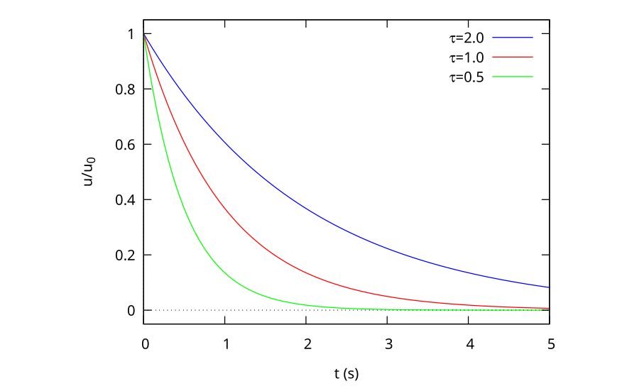
Figure 1: Exponential decay curves for 3 time constants

Other problems will involve an exponential rise from zero to an asymptotic limit, and can be described by the equation

\begin{equation}
\label{orgac57ec5}
u = u_\infty(1 – e^{-t/\tau})
\end{equation}

As a plot, this looks like Fig. 2

ExpRise.jpg

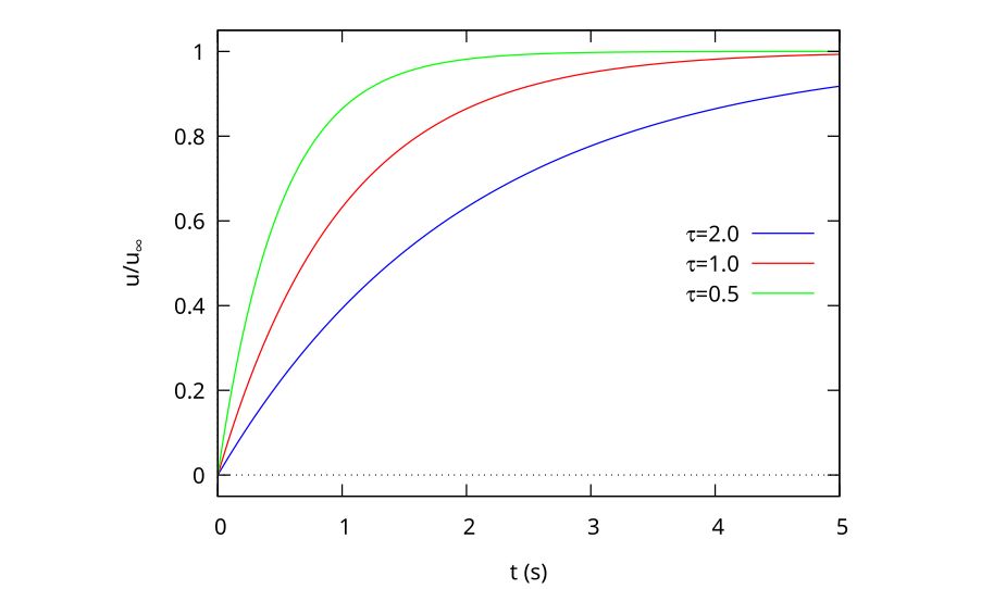
Figure 2: Exponential rise curves for 3 time constants

The most general case of a smooth exponential transition between two non-zero states \(u_0\) and \(u_\infty\) is described by

\begin{equation}
\label{org7a2ccea}
u = u_\infty + (u_0 – u_\infty) e^{-t/\tau}
\end{equation}

Why is the Exponential Form so Important?

As we shall soon see, there are other possible functional forms than Eq. \eqref{org7a2ccea} that we could have chosen that have a similar asymptotic growth or decay behaviour with time. But there is a significant advantage to the natural exponential form because the natural exponential’s derivative is the same as that of the original function, i.e.

\begin{equation}
\frac{d}{dx} e^x = e^x
\end{equation}

or is a constant factor times that function, like

\begin{equation}
\frac{d}{dt} e^{-t/\tau} = -\frac{1}{\tau} e^{-t/\tau}
\end{equation}

This means that the behaviour with time can be described using a single characteristic time parameter, \(\tau\). The physical meaning is that when t = \(\tau\), the solution will have changed by (1 – e^{-1}) = 63.2 per cent of the total change, and every subsequent \(\tau\) will be 63.2 per cent of the remaining change (i.e. 63.2 per cent of 36.8 per cent etc.).

Example: a Falling Rock

Consider the case of a rock falling under the influence of gravity and air drag. The differential equation that describes this behaviour is

\begin{equation}
\label{org885b28d}
m \frac{dv}{dt} = mg – bv^2
\end{equation}

\begin{equation}
[mass \times acceleration] = [gravity force – air drag]
\end{equation}

where \(b\) is the drag coefficient of the body, determined by its shape.

If dropped with an initial velocity of zero, the rock should increase its speed smoothly from zero until reaching a constant velocity when the forces balance, i.e. when

\begin{equation}
mg = bv^2
\end{equation}

or

\begin{equation}
v_\infty = \sqrt{\frac{mg}{b}}
\end{equation}

Although there are a number of ways in which the object could reach the final velocity, the simplest one associated with the gradual balancing of two forces might look like one of those in Fig. 2, with the time constant determined by the mass, the gravitational force and the drag coefficient of the object.

As an aside, notice how in the discussion above I snuck in the assumption that the drag was proportional to the square of the velocity of the object? In fact, this is only true at higher Reynolds numbers and the drag force would be linearly related to velocity at lower speeds. This is one of the dangerous aspects of treating the equation as being independent of the physical problem to be solved. Although the rock would need to be physically very small to have a low enough Re to be proportional to the velocity, I have still seen this form in several example problems in maths textbooks.

While the D.E. in Eq. 5 can be solved directly, we will find an approximate solution using our physical understanding of the problem. This involves 3 basic steps:

  1. making a qualitative sketch (QS) of the solution (we have done this already in Fig. 2)
  2. using this sketch to make a trial function (TF) that describes the equation;
  3. using the TF to determine a design formula for the time constant of the exponential rise

Qualitative Sketch

There are a number of possible ways in which the stone’s velocity can fall as a function of time. Four possibilities are shown in Fig. 3, labelled A through D. Curve A has an overshoot in velocity before reaching a steady value. This sort of thing might happen in an active control system if there is a lag between the controlling force being applied and the effect it has on the speed, but this does not seem likely in the case of air resistance, where the effect is very quick. Curve B has a discontinuity, and does not seem physically realistic. Curve C is smooth and reaches the asymptotic value gradually, so looks like something that would happen. Curve D has a saddle point, and we can’t easily find a reason for that to happen, so it looks like curve C, our exponential growth equation from Eq. \eqref{orgac57ec5}, is the correct functional form.

curves.jpg

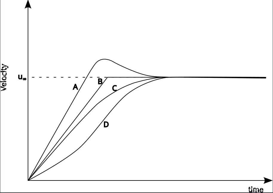
Figure 3: Possible sketches of falling stone velocity

So we are going to assume that this is the general form for the behaviour of the falling stone. Now it may or may not be the exact form, but it has the general behaviour expected of the physical phenomenon. If the equation form is not correct, we can still deduce a time constant that we feel should be reasonably close to the exact time constant.

Trial Function

We choose as the trial function

\begin{equation}
\label{org9876284}
v^* = v_\infty (1 – e^{-t/\tau})
\end{equation}

Here the asterisk indicates that this is a trial function rather than the correct functional description for the behaviour.

Estimating the Time Constant

To get an equivalent time constant, we must substitute our test function Eq. 9 into the differential equation Eq. 5. The derivative is

\begin{equation}
\frac{d v^*}{dt} = \frac{V_\infty}{\tau}e^{-t/\tau}
\end{equation}

and

\begin{equation}
\begin{aligned}
m \frac{dv^*}{dt} &= mg – b v^{*2} \\
m \frac{v_\infty}{\tau} e^{-t/\tau} &= mg – b \left[v_\infty \left( 1 – e ^{-t/\tau}\right) \right]^2 \\
\frac{v_\infty}{\tau} e^{-t/\tau} &= g – g \left( 1 – e^{-t/\tau}\right)^2
\end{aligned}
\end{equation}

Because this is only an approximate solution, there will be a residual \(\mathcal{R}\) relative to the `proper’ solution, which is expressed in terms of the solution’s difference compared with the actual solution:

\begin{equation}
\frac{v_\infty}{\tau} e^{-t/\tau} = g – g \left( 1 – e^{-t/\tau}\right)^2 + \mathcal{R}
\end{equation}

or

\begin{equation}
\label{org68c7fed}
\mathcal{R} = \frac{v_\infty}{\tau} e^{-t/\tau} – g + g \left( 1 – e^{-t/\tau}\right)^2
\end{equation}

The value of \mathcal{R} varies with both the independent variable \(t\) and the time constant \(\tau\). This means we can only force the residual to be zero at certain values of \(t\). If we could make \( \mathcal{R} = 0\) for all values of \(t\), then we would have the correct test function, which is not generally going to be the case.

Collocation at the Half-Way Point

Generally speaking, we want to fix our solution at a point that maintains a good agreement with the actual solution over as much of the solution domain as possible. As the exponential rises from 0 to 1 at \(t = 0\) and \(t = \infty\) respectively, then it makes sense to tie our approximate solution to the actual solution (a method called collocation in the book) at \( e^{-t/\tau} = 0.5\). We do this by setting \( \mathcal{R} = 0\) at this point.

So Eq. 13 becomes

\begin{equation}
\begin{aligned}
\frac{v_\infty}{2\tau} & = g – g (1 – 0.5)^2 \\
& = \frac{3g}{4}
\end{aligned}
\end{equation}

so

\begin{equation}
\label{org7c393cf}
\begin{aligned}
\tau & = \frac{2 v_\infty}{3g} \\
& = \frac{2}{3g} \sqrt{\frac{mg}{b}} \\
& = \frac{2}{3} \sqrt{\frac{m}{gb}}
\end{aligned}
\end{equation}

and the final form of the approximate solution can be determined by substituting for \(\tau\) into Eq. 15:

\begin{equation}
v^* = v_\infty \left(1 – e^{\frac{-t}{\frac{2}{3}\sqrt{\frac{m}{gb}}}}\right)
\end{equation}

Note that in doing this we are not directly solving the differential equation expressed in Eq. 5. We are determining an approximate solution to an equivalent exponential rise problem which will have a very similar time constant. As the time constant is the useful part of the solution, this is really all we need. We are not as concerned with the mathematical correctness of the solution as we are with the physical usefulness.

Note that we didn’t have to collocate at the half-way point. We could have got a different time constant by collocating either earlier or later in the process. The best value across the domain will be the collocation at the half-way point, but if you want a better solution close to \( t = 0\) then you might want to collocate at 0.2 instead, for example. Note that one way of determining how well you have approximated the exact solution to the problem is to determine the collocation at the 0.2 and the 0.8 mark as well as the 0.5 mark. If the time constants are within a factor of 2 of one another across this range, it’s a reasonable approximation across the entire domain, for engineering purposes. Because the collocation process is fairly straightforward, determining the time constant in this way can often provide a good engineering solution with a good idea of its accuracy without ever having to solve the differential equation directly. And if you then go on to solve the exact D.E. then you will have the physical understanding of the problem to back up your solution as a bonus.

`Proper’ Solution and Comparison

In the case of a falling stone, you can directly integrate the equation and, armed with some derivative formulas or a table of standard integrals the solution is given by

\begin{equation}
v = \sqrt{\frac{mg}{b}} \tanh \left(\sqrt{\frac{bg}{m}} t\right)
\end{equation}

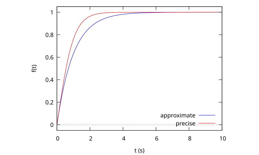
and from Fig. 4, we can see that the hyperbolic tangent form is not exactly the same as the exponential growth form, so our solution is, indeed, approximate. The general behaviour of the two functions is similar, but the exponential distribution is `fuller’ for the same time constant (\(\tau = 1\) in this case).

TanhComp.jpg

Although the physical process is not exactly an exponential growth, we can still determine an effective time constant from the mathematically correct solution, if it’s defined as the time required to grow to 63 per cent of the full velocity, in an analogous way to the exponential growth problem. When we do this we get

\begin{equation}
\tau = 0.745 \sqrt{\frac{m}{gb}}
\end{equation}

compared with the

\begin{equation}
\tau = 0.67 \sqrt{\frac{m}{gb}}
\end{equation}

obtained in Eq. 15 using our approximate form. This is around 11 per cent higher than the approximate solution, and is well within our acceptable limit of 30 per cent.

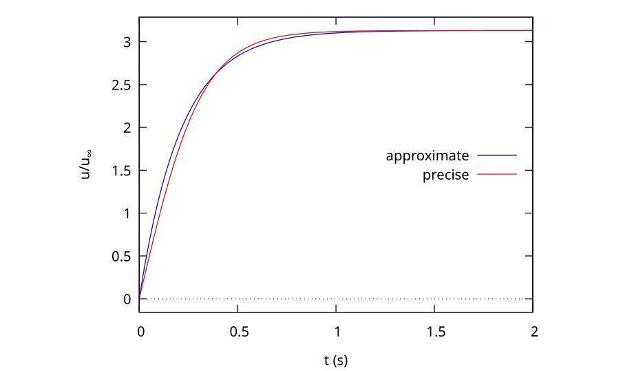
To see the difference between the two solutions, we can plot them both as a function of time, as shown in Fig. 4. It is clear that the approximate solution is very close to the precise solution, which is why the time constants are also close. The collocation point is indicated by the crossover of the approximate and precise solutions. As mentioned, we could collocate earlier to get a better fit to the earlier part of the curve or later to be more accurate later in the history.

In comparing the approximate solution to the mathematically correct one, we see that we have acquired something valuable in exchange for the small inaccuracy. Now we can express the temporal behaviour of the velocity in terms of a physical time constant that just drops out of the analysis because the exponential form is self-similar in a very similar way to how the boundary layer equation is self-similar. But this problem is a lot easier to understand.

Given that we did not solve any differential equations to achieve this approximate result, the fact that both the time constant and the general shape of the curves are so close is an indication fo the power of the technique in a predictive sense, but I think what’s even more impressive is how helpful such a process is for assisting students to understand the mathematical behaviour of the problem using some fairly straightforward physical observations.

Millisecond delay on the STM32F103

Controlling the timer peripherals on the STM32F103 chip can be quite daunting because of the large number of ways in which the timers can be set up and used. However, going to the effort to understand the hardware timers is well worth the effort, as there is so much you can do with the timers, from running servo or stepper motors, to generating delayed pulses on an input trigger, to timing pulse durations to drive an ultrasonic transducer. In this post I thought we would try something relatively simple, while still being useful: a hardware delay word. This is a good way to get the basic idea for how a timer should operate.

Mecrisp does not contain a hardware delay word like us for microsecond-scale delays or ms for longer delays. We can simulate it in hardware by running through an empty DO...LOOP data structure. On my STM32P103 board, a delay caused by counting to around 12000 is enough for a 1-ms delay. But this is imprecise, and system dependent, and also unnecessary when the microcontroller has a hardware timer.

The STM32F103RB has 1 advanced control timer, TIM1, and three other general-purpose (GP) timers (TIM2-TIM4). There isn’t a lot of difference between these timers, although the advanced timer has both the normal output and its complement, whereas the GP timers have only a single output. Other chips in this family also have simple timers with very basic functionality, and if this chip had such a timer we would use it, but it doesn’t, so in this case we are going to achieve our delay with TIM4, one of the general-purpose timers. I could have done this with any of the timers, but the delay is probably best done with the timer you might otherwise use last, so you still have the one advanced timers, and two GP timers for other timing tasks.

To do what we need to do with the general-purpose timers, we first need to have the bit-setting words described in this post: General Forth Words for GPIO On The STM32F103. We will be using the set_bits word to set or reset the appropriate bits on the timer register. So if you have not looked at that article, take the time to do it now, and load the words described there into Mecrisp Forth and Save them to flash, as you will need them to do what I describe below.

What Timers Do

A timer is mostly just a combination of a clock and a counter, with logic that tells the timer what to do when the counter reaches certain pre-set values. All the counters on the STM32F103RB chip are 16-bit counters, meaning that they can count from 0 to 65535. They are able to drive GPIO pins once the counter has reached the pre-set values, or they can start or stop counting when a GPIO pin has changed its state. This allows counters to time input pulses and to generate output pulses with a given duration.

Some of the Chips in the ST family have precision timers with 32-bit resolution for high-resolution timing applications. We won’t discuss them here.

The Important Timer Registers

A general-purpose timer timer has many registers, as outlined in the chip’s manual. Here we refer to the general operations of timers the way the manual does, so TIMx refers to any of TIM1, TIM2, TIM3, TIM4. When searching through the manual, refer to TIMx rather than the individual timer you are interested in. It’s important to note that the Advanced, GP and Simple timers each have their own separate chapters in the chip manual – don’t look at the advanced timer chapter if you are looking at the GP timers! Thankfully, most of the registers are the same for the different types of timers, so most of the information described below also applies for the advanced timers. But there are some small differences in places, so it’s best to look in the appropriate chapter for the timer you are using.

For basic operation, these are the important registers:

  • RCC_APB1ENR: this register turns on the clock for driving the timers. We have already seen the companion register RCC_APB2ENR when we wanted to drive the GPIO clocks.
  • TIMx_PSC: the prescale register. This is a clock divider where the timer takes the system clock frequency and divides it by the value in this register (plus 1) and divides the clock speed by this number. We do this so we can time longer duration pulses. If there were no prescaler then for a clock operating at 72 MHz frequency, we could only count to 65536 at 72 million clock cycles/second, or about 910 microseconds. By scaling down the clock speed, for example if you were to put 71 in this register, you would slow the clock down from 72 MHz to 1 MHz, allowing for longer times to be measured.
  • TIMx_ARR: This is the auto-reload register, a 16-bit register that contains the maximum number the counter will count up to or down from. If counting up, the timer will reset to zero after reaching this number. If counting down, when the counter reaches zero it resets to this number so it can count down again. This register can contain any number from 0 to 65535. If you are generating a continuous waveform with the counter (using something we refer to as pulse-width modulation or PWM) then changing the value in the ARR register is the same as changing the period of the pulse.
  • TIMx_CR1 and TIMx_CR2: The control registers for the timer that determine the type of counter, direction of counter, trigger for the counter to start etc.
  • TIMx_CNT: The register containing the actual count value for the timer.

A Count-down Delay

For the case of a millisecond delay word, all we need to do is set up the timer, set it to count the appropriate number of counts with the correct prescaler, then set it going. If we configure the counter as a down-counter, we must then keep checking to see whether the counter has decreased to zero. If it has, the delay has been completed and the code can continue to do what it was already doing.

The Code

The first thing we do is set the clock speed. The 72MHz word has already been defined in Warp Speed in Mecrisp-Stellaris. Once we are operating at the right speed, we set the variable Freq to that speed. Then we define the base address and offsets for TIM4. Note that you can use the same offset values for any of the timers, so there is no need to redefine them, or to have variables like TIM1_ARR and TIM2_ARR etc. We just need to define the base address of the timer peripheral we want to use and then call the ARR word (for example) to add the appropriate offset for the autoreload register.

72MHz \ Set the system clock to 72 MHz if it wasn't already
72000000 constant Freq \ PSC clock frequency
\ Define registers
$40000800 constant TIM4 
: CR1 ;
: EGR $14 + ;
: PSC $28 + ;
: ARR $2C + ;
: CNT $24 + ;

The next word we define is init_delay. This word turns on the clock for the timer and disables it, allowing the other registers to be changed without affecting the output of the timer. We run this word when loading the file containing this word set to be sure that the timer is clocked but turned off.

: init_delay ( -- )
  RCC_APB1ENR %1 1 2 set_bits \ Turn on clock for timer 4
  0 TIM4 CR1 ! \ Disable the counter
;
init_delay

The next word we define is delay, which is a word that performs a delay for a given number of clock counts. This particular word will work regardless of whether we want delays in microseconds or in milliseconds. The particular type of delay will be defined later, and will be designed to call delay with the appropriate arguments and register settings to give the delay we need. The word delay determines a down-counting single-shot delay, then turns on the counter. A BEGIN...UNTIL loop will wait until the down-counter reaches zero, at which point execution of the word will cease.

: delay ( count -- )
  TIM4 EGR %1 1 0 set_bits 	\ Reinitialise counter and update registers
  DUP TIM4 ARR H! TIM4 CNT H!     \ Set the value in the ARR and CNT Registers
  TIM4 CR1 %11001 5 4 set_bits 	\ Down-count, single shot, enable the counter
  BEGIN 1 TIM4 CR1 bit@ 0= UNTIL
;

The first line uses the set_bits word defined in General Forth Words for GPIO On The STM32F103 to set bit 0 of the EGR register (the UG bit), which resets the counter and the timer registers. Then it takes the count value and stores it in both the ARR and the CNT registers of the timer. The third line sets the parameters of the timer in the CR1 register, and the final line tests for when the timer has decremented to 0. Because the timer has been set to one-shot operation, there is no danger of missing the zero count.

Once the delay word has been defined, it only remains to make words for microsecond and millisecond delays, which just have to set an appropriate value for the prescaler. Now in the STM32 timer chips, the prescaled clock frequency is related to the system clock frequency and the value in the PSC register via the following relationship:

\[ f_{PSC}= \frac{f_{CLK}}{PSC + 1}\]

or, alternatively the value in the prescaler is given by

\[ PSC = \frac{f_{CLK}}{f_{PSC}} – 1 \]

The 1 added or subtracted in these two equations comes from the fact that when the prescaler is set to 0, the frequency of the counter clock is the same as that of the system clock. Knowing this, we can define our microsecond and millisecond delay words, us and ms, respectively:

: us ( n -- )
  DUP 60001 < IF
    Freq 1000000 / 1- TIM4 PSC H!
    delay
  ELSE CR . ." us delay too long.  Use ms instead."
  THEN ;
: ms ( n -- )
  \ Times up to 30 seconds
  DUP 30001 < IF 
    Freq 2001 / TIM4 PSC H!
    2* 1- delay
  ELSE CR . ." ms Delay too long."
  THEN ;

Using this setup, we can type something like 200 ms to generate a delay of 200 milliseconds, or 1000 us to generate a delay of 1000 microseconds. Execution will pass to the next word to be evaluated once the delay word has completed by counting down to zero.

Note that the ms word halves the prescaler and doubles the number of counts, because otherwise the prescaler value would be 72000, which is larger than can be stored as a 16-bit number. I have had to modify the counter value a little from the expected value to remove an offset, but it provides an accurate delay between 1 and 30000 ms.

We can test the behaviour of these words by writing some test words that turn on and off a GPIO port pin, before and after execution of the delay. For example, the following are words to test the ms and us delay words:

: mstest ( n1  -- ) \ test for ms delay
  GPIOC enable
  GPIOC 10 ppout
  GPIOC 10 GPon
  ms
  GPIOC 10 GPoff ;
: ustest ( n1  -- ) \ test for us delay
  8 MAX 7 - \ remove offset of 7 us
  GPIOC enable
  GPIOC 10 ppout
  GPIOC 10 GPon
  us
  GPIOC 10 GPoff ;

The 8 Max 7 – ensures that the 7 microsecond offset from executing the word is removed from the count, and that the delay is a minimum of 8 microseconds long. The delay in the code execution prevents us from using a lower delay than this.

Typing something like 2 mstest will generate a pulse that is 2 ms long on PC10. This will result in a waveform that looks like the one below:

2msDelay.png

Note that the utest word removes 7 microseconds from the count. This is done to compensate for the time required to execute the Forth words, which becomes significant at small delays.

Org-mode Signature Code

I’ve been trying to learn a little elisp lately, and have written a useful routine that I thought someone might like. It’s interesting because it uses both elisp and org-mode tables.

Lately I have been setting up mu4e to read my personal email. As part of using that I wanted to have a signature that would generate a wise saying from a country, but to make it a bit more interesting I wanted the signature to choose a randomly selected saying from a different country each time I generated the signature.

I have an org-mode file that contains a two-column table. The first column contains the country and the second contains the quote.

#+NAME: SayingsTab
| Afghanistan           | Don't show me the palm tree, show me the dates                                      |
| Afghanistan           | No one says his own buttermilk is sour                                              |
| Afghanistan           | What you see in yourself is what you see in the world                               |
| Africa                | The tree that has been axed will never forget                                       |
| Albania               | Don't put gold buttons on a torn coat                                               |
| Albania               | Patience is the key to paradise                                                     |
| Albania               | When you have no companion, consult your walking stick                              |
| Algeria               | Do bad and remember, do good and forget                                             |
| America               | A pessimist is a person who has lived with an optimist                              |
| Armenia               | You cannot start a fast with baklava in your hand                                   |
| Australia             | There are none so deaf as those who will not hear                                   |
|-------------------------------------------------------------------------------------------------------------|
#+name: quote
#+begin_src elisp  :exports results :var sayings=SayingsTab
	(defun genquote()
      "Generate a random quote from an org-mode table.
  The table contains the country name in col 0 and the quote in col 1.
  Add more quotes to the table as needed, the function
 selects from the current number of rows."
	(interactive)
   (let ((selection  (nth (random (length sayings)) sayings)))
	  (message "As they say in %s, \"%s\"." (car selection) (cadr selection))))
   (genquote)
#+end_src

Running the source block here generates a random quote from the list in the table as a message. Hitting C-c C-c in the code will run it and generate a quote like

As they say in America, "A pessimist is a person who has lived with an optimist".

I like using the org-table because the new items can be sorted alphabetically, and its easy to add new sayings when I find them.

What I’d like to be able to do is to load the org table using an elisp function and then do the same thing as part of a signature-generating function. Currently I can’ do that, but I can read the text from a tab-delimited text file. Fortunately, I can generate the tabular data that can be read by elisp by putting the point at the table and using the M-x org-table-export command. I save the table to a tab-delimited file called sayings.txt whenever I add to the org-table.

Then in my init.el file, I define the following elisp function to generate an email signature using the data in the text file.

(defun signature()
   "Generates a random quote from a tab-delimited file for use as an email signature quote. 
	       Table of quotes is in ~/ownCloud/Org/sayings.txt
	       The tab-delimited table contains the country name in col 0 and the quote in col 1.
	       Add more quotes to the table as needed, the function
	       selects from the current number of rows."
   (interactive)
   (setq sayings (read-lines "~/ownCloud/Org/sayings.txt"))
   (setq sel (nth (random (length sayings)) sayings))
   (insert "\n-- \n" "John Doe \n \n" "john.doe@google.com \n" "Ph: 867 5309 \n")
   (insert "As they say in ")
   (insert (remove-trailing (car (split-string sel "\t" t))) ", '")
   (insert (remove-trailing (cadr (split-string sel "\t" t))) "'. \n")
   )

This should produce something like

-- 
John Doe 
john.doe@google.com 
Ph: 867 5309 
As they say in Malaysia, 'One buffalo brings mud and all the herd are smeared with it'. 

where the last line is the randomly generated quote. So then, when I’m editing my email, I just need to call the signature function when editing an email in mu4e and I get my signature with a new quote every time.

If you know how to read direct from the org-table, rather than from a text file, I’d love to know how you do it, as that would remove the need to update the table from time to time.

Maxima and IMaxima on Emacs

Sometimes (actually less frequently than I should) I try to do some maths. I tend to do more of it in teaching than in my research, as my research is mostly experimental and usually I’m using someone else’s maths. Most of my research calculations are numerical, and J works really well and efficiently for these sorts of things. However sometimes you need to use analytical maths, and when that happens and you forget the calculus you learned as an undergraduate, then computational algebra systems (CAS) can be very useful.

Probably the most well known CAS is mathematica, which became popular at the time when Macintosh GUI-based applications were coming out, but mathematica was at least in part the outgrowth of existing primarily text-based CASs such as Macsyma, Derive and others. Many of these started their lives as commercial packages, but were either discontinued because of mathematica’s dominance of the commercial space (like MathCad, which I used during my PhD) or were open-sourced. There are several open-source CASs around now, with the most common being maxima, SageMath and Fricas. Here I’m going to be talking about maxima.

Maxima is a descendent of Macsyma, a lisp-based CAS first written in the 1960s and released into the public domain. I have chosen this CAS, as it has good hooks into emacs, in particular a nice plugin that is part of the maxima package called imaxima.

There is another package called wxmaxima that contains a GUI interface to maxima, and many people use this because it has lots of nice icons and is easy to use. However, as an emacs user, I prefer to use the maxima REPL within an emacs buffer, and fortunately maxima comes with a file imaxima.el that allows all the power of maxima to be available from an emacs buffer.

Installation

First, install maxima itself. On linux systems, use your favourite package manager (eg apt on Debian systems). In my case, I use Manjaro, so I use pacman as the package manager. You can see the maxima-based packages using

pacman -Ss maxima

This produces

extra/maxima 5.46.0-2 [installed]
    A sophisticated computer algebra system
extra/maxima-ecl 5.46.0-2 [installed]
    ECL backend for Maxima
extra/maxima-fas 5.46.0-2
    Maxima FAS module for ECL
extra/maxima-sbcl 5.46.0-2 [installed]
   SBCL backend for Maxima

on my system. As I use sbcl, maxima-sbcl provides a back-end for that Lisp interpreter. Installation on my system is done typing

pacman -S maxima maxima-ecl maxima-sbcl

on the command line.

If you have the locate command installed (it can also be installed via pacman on Manjaro) then after typing

sudo updatedb

on the command line, followed by

locate imaxima.el

produces

/usr/share/emacs/site-lisp/maxima/imaxima.el

as an output. Then, to install imaxima, I put the following lines in my init.el file

;-----------------------------------------------------------------------
; imaxima - interactive computational algebra system
;-----------------------------------------------------------------------
(push "/usr/share/emacs/site-lisp" load-path)
(autoload 'imaxima "imaxima" "Maxima frontend" t)
(autoload 'imath "imath" "Interactive Math mode" t)
(setq imaxima-fnt-size "Large")

You may need to change the path based upon your locate command. These commands run the imaxima and imath functions that allow interactive use of imaxima and inline insertion of latex-quality equations in the output.

Examples

Once installed, typing M-x imaxima starts the interactive shell for imaxima. I’m not even going to try to make a maxima tutorial here, as there are already several available. Figure 1 contains an example of calculation of normal unit vectors for a vector function at a given location. Note that the equations are nicely typeset.

imaxima.png

Figure 1: Maxima session showing vector calculations

And of course no demo would be complete without the arbitrary plotting of a pretty 3D function, in this case a hyperboloid.

MaximaFuncPlot.png

Figure 2: Maxima with pretty plot

The M-x maxima command also works if the maxima package is installed (see next section), but the output is in text form, which is not as aesthetically appealing. The text below is the equivalent maxima output to that in Figure 1 for imaxima.

(%i92) r(t) := [t, cos(t), sin(t)];
(%o92)                    r(t) := [t, cos(t), sin(t)]
(%i93) limit(r(t), t, 2, plus);
(%o93)                        [2, cos(2), sin(2)]
(%i94) limit(r(t), t, 3, minus);
(%o94)                        [3, cos(3), sin(3)]
(%i95) diff(r(t), t);
(%o95)                       [1, - sin(t), cos(t)]
(%i96) define(rp(t), diff(r(t), t));
(%o96)                  rp(t) := [1, - sin(t), cos(t)]
(%i97) load(eigen);
(%o97)          /usr/share/maxima/5.46.0/share/matrix/eigen.mac
(%i98) uvect(rp(t));
                     1                           sin(t)
(%o98) [---------------------------, - ---------------------------, 
                2         2                    2         2
        sqrt(sin (t) + cos (t) + 1)    sqrt(sin (t) + cos (t) + 1)
                                                            cos(t)
                                                   ---------------------------]
                                                           2         2
                                                   sqrt(sin (t) + cos (t) + 1)
(%i99) trigsimp(%);
                             1       sin(t)   cos(t)
(%o99)                   [-------, - -------, -------]
                          sqrt(2)    sqrt(2)  sqrt(2)

It does the job, but the text is harder to read, at least for me, than the nicely typeset output.

Other Computer Algebra Systems

In addition to imaxima, there is a package on ELPA called maxima, which installs a major mode for editing maxima files. Also there is an interface to the Fricas CAS, called Frimacs, which I have not used, but which is worth investigating. Fricas is descended from Axiom, another commercial CAS, and is apparently strong at automatic integration of functions.

Conclusion

There is no question, these CASs can be very useful, either for learning algebra and calculus, or for using them in mathematics, physics and engineering applications. They can be used for anything from a simple calculator alternative (although M-x calc is much better for this) to a solver of integrals, derivatives and linear algebra problems, and for plotting of functions. Often the output of calculations is not simplified in the way one might expect when doing it by hand, but there are simplifying commands that can get around those limitations. It’s also a great tool when I can’t remember my integration techniques. I’ll be trying to use it more in my maths calculations in future now that it’s set up.

General Forth Words for GPIO On The STM32F103

This blog entry goes into the design of a Mecrisp Forth wordset that allows you to program the GPIO ports. This is typically one of the first things one learns to do on a microcontroller, and is usually taught by getting one or more LEDs to flash. We will hook up LEDs to the PC10 and PC8 pins of the STM32P103 board and write some code to get them to flash.

If one were to write a code to do this in an algol-derived programming language like C or the C-like language used in the Arduino programming environment, one would usually write code that involves calls to built-in libraries. For an Arduino, the code might look something like:

#define LED PC10
void setup() {
  // initialize digital pin LED_BUILTIN as an output.
  pinMode(LED, OUTPUT);
}
 
// the loop function runs over and over again forever
void loop() {
  digitalWrite(LED, HIGH);   // turn the LED on (HIGH is the voltage level)
  delay(200);                       // wait for 200 ms
  digitalWrite(LED, LOW);    // turn the LED off by making the voltage LOW
  delay(200);                       // wait for 200 ms
}

This code sets up port C pin 10 in the function setup as an output using a function called pinMode, and uses a separate function loop which, in turn, calls a function called digitalWrite to set the pin to high or low with a delay set by a call to the function delay, in this case of 200 ms. One may also need a function to turn on the clock to port C if it can’t already be assumed to be on.

Presumably one would include calls to these functions within a loop in a function main to complete the program. This is not too difficult to follow, if you ignore all the infrastructure like semicolons and explicit type declarations. And it’s nice to be able to call these pre-built functions, provided you can remember the function name someone else decided upon, and that you don’t want to do things that are not catered for in the function. For example, the pinMode function does not have an input parameter that allows you to set the clock speed of the GPIO pins, which is an option that is available on the chip. Of course you could write your own pinMode function, but perhaps other functions in the library would use the original pinMode function with a different clock speed. Because you didn’t write the code, you don’t easily know what was done in the library.

Forth encourages programmers to look at a problem like this differently. Rather than forcing the programmer’s application to always look like the syntax of the programming language, Forth makes it very easy for a programmer to make words that define a domain-specific language that is tailored to solving that particular problem. By combining the concept of the dictionary and the implicit passing of parameters on the stack, this domain-specific language can be made to look like a set of commands to the microcontroller that are set up to control any GPIO port. And with a little thought, they can be made quite general.

Pre-reading

Before we can make the generalised GPIO words, we need to make some words that allow us to save bit patterns to registers without changing the remaining bits in those registers. These nondestructive bit setting and resetting words were introduced previously here in a previous blog entry. It’s best to go through that and make sure you understand those words before going any further.

How to control GPIO

To get a GPIO port working you need to do three things:

  • Turn on the clock
    • This is done using the RCC_APB2ENR clock enabling register
  • Set the pin on the port to be an input or an output
    • This is done using the GPIOx_CRL (for pins 0-7 on a given port) or GPIOx_CRH (for pins 8 through 15).
  • Write or read the value of the bit(s) we are interested in, i.e.
    • Set or reset the bit in the GPIOx_ODR register to turn an output on or off, or
    • Read the value of the pin in the GPIOx_IDR register if you want to know if an input is on or off.

GPIO Registers and Where to Find Them

One of the neat things about the design of the registers in the STM32F103 chip is that each of the GPIO ports is separated by a consistent offset ($400) and each of the control registers for any port is at the same offset from the base address of that port. This consistency means that we are able to write generalised words that can be used to set any aspect of the behaviour of any of the GPIO pins on any of the ports.

The GPIO ports in the STM32F103 have addresses that can be found in the STM32F103 reference manual, in Section 3.3. All of ports A through E are in consecutive peripheral base addresses, as shown in the table below:

Port Base Address
A $4001 0800
B $4001 0C00
C $4001 1000
D $4001 1400
E $4001 1800

Each of these ports will have several registers, separated by 4 bytes from each other, that control the behaviour of these registers. In our GPIO library we will concentrate only on the most used of these registers, though once you know how to make the words, it will be easy to add words to change the other registers if necessary.

For the GPIO control we are interested in, we will be setting values in the registers GPIOx_CRL, GPIOx_CRH, GPIOx_IDR and GPIOx_ODR. Although there are other registers such as the GPIOx_BSRR set/reset register and the GPIOx_LOCKR lock register, I don’t use them, so won’t be using them in this wordset. I have also avoided the AFIO alternate function registers here, because we will come to them when using the timers later on.

In addition to the GPIO registers we also add the port clock setting register, RCC_APB2ENR that controls the clock of the five ports. By default, my Mecrisp has ports A, B and C switched on, so I don’t tend to set it. But for the sake of the exercise we will provide words that use that clock control register as well to turn on the ports.

Domain-specific Language Design

Before writing a Forth code, I like to imagine how I would call the words to operate the GPIO. This gives me a starting point for the implementation of the wordset itself, because I then know what the final words should look like. I would like to be able to use the same words to control any of the ports, which means that I would need to have a word that indicates the base address of the port, with words like GPIOA, GPIOB etc returning the base addresses of those ports. This allows me to write words that permit commands like GPIOA enable to enable the clock for GPIO port A.

Control commands based upon words like this would look something like

GPIOC enable  	\ enable port C
GPIOC 10 ppout 	\ set port to push-pull output (50 MHz)
GPIOC 10 GPon	\ turn on GPIOC pin 10
GPIOC 10 GPoff	\ turn off GPIOC pin 10

Words like this can then be included in more complex words such as lflashes to flash a particular pin a certain number of times

GPIOC 10 20 lflashes	\ flash GPIOC pin 10 20 times

and extended to do still more complex things like running light displays, all building upon these primitive port control words. At this point it’s worth comparing the Forth control method with the Arduino code at the start of this blog entry. Once the words have been made, the Forth code produces a direct command language available to the Forth user that looks a little like Forth, but a lot like a language designed to control GPIOs (albeit with an infix way of inputting data). In contrast, the Arduino code always carries the baggage of looking like the programming language it was implemented in. This is, I think, one of the strongest arguments for the use of Forth as a programming environment for microcontrollers. For some, the fact that the Arduino code always looks consistent with other Arduino code is an advantage because only one syntax needs to be learned. I have always thought the Forth way of doing things is cleaner-looking when done properly.

Building the Wordset

Now that we know the way we want to control the GPIO, we need to make words that allow us to develop those words. In other words, we are designing the application from the top down and implementing from the bottom up, once we know what the top-level words look like.

Initialising the Port(s)

The initialisation word switches on the clock for the port. This is done by setting bits in the RCC_APB2ENR register, shown in Fig. 1.

RCC_APB2ENR.png

Figure 1: RCC_APB2ENR Register

This register contains the clock enable bits for a number of peripherals, including all the GPIO ports. Notice that GPIOA through GPIOG are all consecutive (although the STM32F103RBT6 in the Olimex STM32P103 board that I am using only has ports A through E).

So to turn on the clock for a given port, we need to set bit 2 for port A, bit 3 for Port B etc. Assuming we are using the port address as the alias for PortA etc, we need a way to convert the address to the offset. We use the fact that the port addresses are $400 apart to subtract the address from port A’s address, divide by $400 and add 2 to determine the bit position we need to switch on.

First, we make constants for the base addresses of each port and for the RCC_APB2ENR register:

\ Address locations
$40010800 CONSTANT GPIOA 
$40010C00 CONSTANT GPIOB
$40011000 CONSTANT GPIOC
$40011400 CONSTANT GPIOD
$40021018 CONSTANT RCC_APB2ENR

Now we make the enable and disable words that allow us to set or reset the clock for a given port using the set_bits word we declared in the previous blog entry on non-destructive bit setting:

\ Application words 
: enable ( aPort -- ) 
  GPIOA - $400 / 2 + 
  RCC_APB2ENR SWAP 
  1 1 ROT
  set_bits ;         \ Turn on the clock
: disable ( aPort -- ) 
  GPIOA - $400 / 2 + \ Set location to shift to 
  RCC_APB2ENR SWAP
  0 1  ROT
  set_bits ;         \ Turn on the clock

This allows us to use commands like GPIOA enable or GPIOC disable to enable or disable any of the ports. One should be careful about disabling whole ports, as sometimes these ports can be used for other peripherals. For example, USART1 is driven by pins on GPIO port A and switching that off may stop Forth from communicating with the terminal program!

Once we can enable the port, we next have to be able to determine whether a pin is an input or an output. To do this, we need to declare the positions of the control registers for this particular port. Because the designers of the STM32F103 were nice enough to make the control register offsets the same for all the ports, we can define the registers as offsets from the base address.

\ Register offset definitions
\ NB aPort is the address of the port (eg GPIOA, as defined above) 
: CRL ( aPort -- aPort + CRL ) ;
: CRH ( aPort -- aPort + CRH ) $04 + ;
: IDR ( aPort -- aPort + IDR ) $08 + ;
: ODR ( aPort -- aPort + ODR ) $0C + ;

Thus, the commands GPIOA ODR will provide the address of the output data register for GPIOA, and GPIOE ODR provides the equivalent address for GPIOE. This means that you don’t need to declare constants for each of the registers of each of the ports separately.

To set a particular pin of a particular port to be an input or an output. To do this, we must set 4 bits: 2 CNF bits and 2 MODE bits. These 4 bits are indexed by 4 bits per pin, stretched over 2 registers – GPIOx_CRL for pins 0–7 and GPIOx_CRH for pins 8–15. The two lower MODE bits determine whether the pin is an input or an output while the CNF bits outline what kind of input or output the pin is. The arrangement is shown in Fig. 2 for the CRH register.

GPIOx_CRH.png

Figure 2: GPIOx_CRH register

MODE GPIO type
00 Input
01 10 MHz output
10 2 MHz output
11 50 MHz output
CNF GPIO type
If input
00 Analog
01 Floating
10 Pull up/pull-down
11 Reserved
If output
00 General purpose push/pull
01 General purpose open drain
10 Alternate function push/pull
11 Alternate function open drain

Any given pin of any given port can be set with any combination of these 4 bits, depending on how the GPIO is to operate. To make this work in a general way, I have made a word called GPset that takes the port address, pin number and the 4-bit string from the table above and uses our non-destructive set-bits word to set the appropriate 4 bits in the CRL or CRH register. We can then make words describing the type of input or output that you would like that pin to be, using the bit pattern with the call to GPset. The GPset word must choose whether the CRL or CRH register must be written to, based upon the pin number on the stack. This is done with an IF ... ELSE ... THEN statement.

: GPset ( aPort pin# porttype -- )
  \ Set a pin to output
  \ porttype is a 4-bit pattern
  >R 
  DUP 7 >
  IF 7 - SWAP CRH SWAP ELSE 1+ SWAP CRL SWAP THEN     
  4 * 1-
  R> 4 ROT  set_bits  ;
: ppout     ( aPort pin# -- ) %0011 GPset ; 	\ Set port pin to push-pull output, 50 MHz
: ppout2MHz ( aPort pin# -- ) %0010 GPset ; 	\ Set port pin to push-pull output, 2 MHz
: afout     ( aPort pin# -- ) %1011 GPset ; 	\ Set port pin to AF output, 50 MHz
: ppin      ( aPort pin# -- ) %1000 GPset ; 	\ Set port pin to push-pull input
: ain       ( aPort oun# -- ) %0000 GPset ; 	\ Set port pin to analog input

We can then issue commands like GPIOC 10 ppout to set pin 10 of GPIO port C to a 50 MHz push-pull output, or GPIOB 8 ppin to set pin 8 of GPIO port B to an input.

Once we can switch the ports on or off and declare the type of input or an output for a given pin of a given port, all that remains is to read from (for an input pin) or write to (for an output pin) the port. The reading or writing are done with the lower 16 bits of the IDR (for inputs) or ODR (for outputs) register. Again, we use set_bits for the setting, but for the reading we use LSHIFT for reading the port, using bitwise AND to set all the other bits to zero, leaving either a true (for a 1) or false (for a 0) at the bit position of interest.

: GPon ( aPort pin# -- )
  \ Turn on a pin for an output port
  SWAP ODR SWAP %1 1 ROT set_bits ;
: GPoff ( aPort pin# -- )
  \ Turn off a pin for an output port
  SWAP ODR SWAP %0 1 ROT set_bits ;
: GPon? ( aPort pin# -- fl )
  \ Check to see if an input is switched on
  SWAP IDR @ 1 SWAP LSHIFT AND = ;

And that’s pretty much all that’s needed to get a general-purpose GPIO wordset working that allows bits to be manipulated as needed. The remainder of the file provides a demonstration of the operation of this wordset in making simple LED flashing words. Set up a red LED and a 220 Ohm resistor going from pin 8 and pin 10 to ground. The setup for pin 10 is shown in Fig. 3.

GPIOLED.png

Figure 3: Setup for LED on Pin 10 of GPIOC

The setup here is done with the port driving pin 8 and pin 10 directly from the port. The port outputs can sink enough current to drive a LED, though it’s probably better to connect the anode to the +3.3V supply on the board and the ground-connection to the port. If you connect the ports this way, you can drive more current as the port is sinking to ground.

The rest of the code provides words that can flash an LED a given number of times using the lflashes word, or can flash the two outputs using the alternate word. Note that lflash is built upon GPon and GPoff, lflashes and alternate are built upon lflash. The ms word used here employs a software loop to generate the delay for the pin flash. It’s set up for a 72 MHz clock speed, and the delay multiple scale may need to be changed for a lower value if the clock speed is lower. In a future post we’ll work out how to make a more accurate timing word using the STM32F103’s built-in timers, but this is sufficient for illustration. The comments at the end of the code show you how this domain-specific GPIO language can be used to control input and output ports.

I hope this short example shows you how Forth can take some very simple primitive words and develop a language specifically tailored to a particular interactive programming task. The full source is reproduced below.

\ GPIO General Access Wordset
\ This is an example of how you can use Forth to make a language for 
\ operating your GPIO ports on the STM32F103 processor
\ Note that this particular code only deals with setting an entire
\ high or low part of a port to an input or an output
\ Also note that the ms word is highly dependent on the clock speed
\ Note that these words can be used with any of ports A, B, C and D
\ and can configure any output.
\
\ Sean O'Byrne 03/2022
\ Code released under terms of the Gnu Public Licence Version 3

\ Address locations
$40010800 CONSTANT GPIOA 
$40010C00 CONSTANT GPIOB
$40011000 CONSTANT GPIOC
$40011400 CONSTANT GPIOD
$40021018 CONSTANT RCC_APB2ENR

\ Register offset definitions
\ NB aPort is the address of the port (eg GPIOA, as defined above) 
: CRL ( aPort -- aPort + CRL ) ;
: CRH ( aPort -- aPort + CRH ) $04 + ;
: IDR ( aPort -- aPort + IDR ) $08 + ;
: ODR ( aPort -- aPort + ODR ) $0C + ;

\ Utility words

: ones ( n -- %11..1 )
  \ Generate a binary number consisting of n 1s
  1 SWAP 1- 0 ?DO 2 * 1 + LOOP ;

: pos_shift ( nbits pos -- nbits shift# )
  \ Determines the number of bits to shift given the position of the MSB
  \ and the number of bits
  OVER - 1+ ;

: not_mask ( nbits shift -- shift mask )
  \ Generate mask consisting of 1s everywhere but where we want to
  \ change bits
  SWAP ones OVER LSHIFT NOT ;

: set_bits ( addr %n nbits pos -- )
  \ Stores a bit pattern bits starting at a given bit position at address adr
  \ bits consists of nbits 1s and 0s at position pos in a 32-bit word.
  \ Non-intrusive for all other bits.
  \ Usage:
  \        GPIOC CRH %0011 4 7 set_bits
  \ This would place the 4-bit pattern %0011 at bit position 7 in GPIOC_CRH.
  \ The word b counts the bits (including leading zeros) in the binary number.
  \ Note that b can only be used interactively, not within a word definition.
 
  pos_shift \ Determine number of bits to shift pattern
  not_mask  \ Set bit pattern to AND with
  >R
  LSHIFT    \ Set bit pattern to OR with
  OVER @
  R>
  AND       \ AND with mask to get 0s at correct bit positions
  OR        \ OR with bit pattern to nonintrusively set
  SWAP ! ;  \ Store new bit pattern at address

\ Application words 
: enable ( aPort -- ) 
  GPIOA - $400 / 2 + 
  RCC_APB2ENR SWAP 
  1 1 ROT
  set_bits ;         \ Turn on the clock

: disable ( aPort -- ) 
  GPIOA - $400 / 2 + \ Set location to shift to 
  RCC_APB2ENR SWAP
  0 1  ROT
  set_bits ;         \ Turn on the clock

: GPset ( aPort pin# porttype -- )
  \ Set a pin to output
  \ porttype is a 4-bit pattern
  >R 
  DUP 7 >
  IF 7 - SWAP CRH SWAP ELSE 1+ SWAP CRL SWAP THEN     
  4 * 1-
  R> 4 ROT  set_bits  ;

: ppout     ( aPort pin# -- ) %0011 GPset ; 	\ Set port pin to push-pull output, 50 MHz
: ppout2MHz ( aPort pin# -- ) %0010 GPset ; 	\ Set port pin to push-pull output, 2 MHz
: afout     ( aPort pin# -- ) %1011 GPset ; 	\ Set port pin to AF output, 50 MHz
: ppin      ( aPort pin# -- ) %1000 GPset ; 	\ Set port pin to push-pull input
: ain       ( aPort pin# -- ) %0000 GPset ; 	\ Set port pin to analog input

: all_outputs ( aPort -- ) DUP CRH $33333333 SWAP ! CRL $33333333 SWAP ! ;
: all_inputs  ( aPort -- ) DUP CRH $88888888 SWAP ! CRL $88888888 SWAP ! ;

: GPon ( aPort pin# -- )
  \ Turn on a pin for an output port
  SWAP ODR SWAP %1 1 ROT set_bits ;

: GPoff ( aPort pin# -- )
  \ Turn off a pin for an output port
  SWAP ODR SWAP %0 1 ROT set_bits ;

: GPon? ( aPort pin# -- fl )
  \ Check to see if an input is switched on
  SWAP IDR @ 1 SWAP LSHIFT AND = ;

\ LED Flashing Routines
\ Here are some example words to make LEDs flash

\ Setup for LED flashing
GPIOC enable
GPIOC 10 ppout
GPIOC 8 ppout
0 GPIOC ODR H!

200 VARIABLE time \ flash delay time, in ms
12000 VARIABLE scale

\ Software ms loop 
: ms scale @ * 0 do loop ; \ change number to get accurate ms timing

: pulse ( n -- ) GPIOC 10 2dup GPon rot ms GPoff ;

: lflash ( aPort bit_pattern -- ) \ Flashes PC10 for the appropriate number of ms
  2DUP GPon time @ ms GPoff time @ ms ;

: lflashes ( aPort pin# n -- ) \ Flashes PC10 n times
  0 ?DO 2DUP lflash LOOP 2DROP ;

: alternate ( n -- )
  0 ?DO GPIOC 10 lflash time @ ms GPIOC 8 lflash time @ ms LOOP ;


\ Now you can try the following after hooking up an LED and resistor to 
\ port C pin 10 and another to port C pin 8...
\ Example usage below
\ GPIOC port_enable
\ GPIOC all_outputs
\ GPIOC 10 GPon
\ GPIOC 10 GPoff
\ GPIOC 10 lflash
\ GPIOC 8 lflash
\ GPIOC 10 20 lflashes

Hypersonic Tesla

As you might know, Tesla went and launched one of their roadster vehicles into space some time back. I’m still not sure why, but I guess it was because Elon Musk could.  So, in that spirit, because we have a facility that can generate hypersonic flow, my colleague Harald and I decided to see what it would look like if an alien decided to drive it back to Earth… So if you are curious, this is what a Tesla roadster would look like if it were entering the upper atmosphere at Mach 10.  Harald used a technique called colour schlieren to visualise the shock waves around the vehicle, and front-illuminated the vehicle so it looks like the vehicle rather than a shadow.  The colours near the end of the video have nothing to do with the hypersonic flow, but are either caused by the high temperature reacting with the paint on the car or is old rubidium that we used for previous experiments in the tunnel, still left over from those experiments.

The car was a little toy Matchbox Tesla Roadster model.  Just a bit of fun, but a nice illustration of how interesting and complex hypersonic flow can be, and a showcase for Harald’s talent!


Non-destructive Bit Setting in Mecrisp Stellaris Forth

Doing pretty much anything involving a peripheral on the STM32F103 microcontroller (or on most microcontrollers for that matter) involves putting ones or zeros into registers or reading the registers to see which bits are ones or zeros. The simplest way to do this is to write or read the number you want to write into the register. In Forth, this is done using the ! and @ words, respectively.

For example, $33333333 $40011000 ! stores the appropriate bit pattern to turn all the lower 8 pins of the general-purpose input-output port C (GPIOC) to be 50 MHz push-pull outputs, by setting all the bits of the GPIOC_CRL register located at address $40011000.

While this is easy to do, it has the disadvantage that whatever used to be in that register has now been obliterated by the $33333333. Often we just want to change the state of one pin of one of our GPIO ports without interfering with the others. This is particularly true of ports that operate more than 1 peripheral… you don’t want to lose your serial connection when changing a GPIO port.

So what we need is the ability to set 1 or more bits in a register without changing any of the others. An example of this sort of requirement is the setting of the GPIOx_CRH or GPIOx_CRL register to determine whether a particular pin in a GPIO port is an input or an output. This is done by setting 4 bits in this register. Which particular 4 bits to set, and indeed which of the CRL or CRH registers to set them in, will be different depending on the pin you want to set and the port containing that pin.

As an example, say that we want to set pin 10 of GPIO port C to be a push-pull output operating with a clock speed of 50 MHz. As it’s higher than pin 7, the appropriate register to set is GPIOC_CRH, located at $40011004 on the STM32F103 chip. The diagrammatic representation of this register, based upon the chip manual, is shown in the figure below

GPIOx_CRH.png

Each of pins 8 to 15 of the particular port (in this case port C) is controlled using 4 bits. The lower 2 bits are called mode bits and determine whether the port is an input or an output, and what speed it outputs to if it is the latter type. The upper two bits provide further characteristics of the input/output port. The lowest 4 bits control pin 8, the next higher 4 bits control pin 9 and so on.

For this case, if we want to set pin 10 to be a push-pull output at 50 MHz clock rate, we need to set bits 8-11 of this register to the binary number %0011. But we want to achieve this without changing the values of any of the other pins in this half of the port. The desired change in the port is shown below.

GPIOC_CRH_InitFinal.png

The x’s indicate either 0 or 1 values in that bit position.

Bitwise Logic

So if we want to set just these bits then we have to recall some bitwise Boolean logic operations. Specifically we will recall three important bitwise operations: NOT, AND and OR.

NOT is the simplest of these, as it only operates on single bits, reversing their value at every bit position. Thus, 0s become 1s and 1s become 0s. The truth table for the NOT operation looks like this:

NOT

Input Output
0 1
1 0

AND and OR both operate on two numbers, one bit at a time.

AND

Input 1 Input 2 Output
0 0 0
0 1 0
1 0 0
1 1 1

OR

Input 1 Input 2 Output
0 0 0
0 1 1
1 0 1
1 1 1

In the case of AND, the only time a bit is not set to 0 is when both input bits are 1. Similarly, for OR, the only time a bit is not set to 1 is when both input bits are 0.

We can also use the XOR operation to toggle bits where that is needed:

XOR

Input 1 Input 2 Output
0 0 0
0 1 1
1 0 1
1 1 0

Looking at the truth table for AND, you can see that *AND*ing a bit with 0 always sets it to 0, while *AND*ing a bit with 1 leaves the original bit unchanged. Similarly, ORing a bit with 1 always sets it to 1 while *OR*ing a bit with 0 leaves the original bit unchanged.

Thus, if I want to set a bit within a number to 1 while not changing the value of any of the other bits, I need to have a number of the same length with 0s everywhere except at the position that I need to set to 1.

To set a bit to 0, I need the opposite. I need to AND each bit with a 1 where I want to leave the bit unchanged and to AND with a 0 at the location of the bit I want to reset to 0. To do this conveniently, one typically puts a 1 at the location to reset, performs the NOT operation to all the bits, turning that bit to 0 and all the other bits in the number to 1s, then AND with the original value. By doing this, all the other bits are unchanged because they are being *AND*ed with 1 and the bit you wish to reset is always 0 regardless of whether it was a 0 or a 1 because you are *AND*ing that bit with 0. This takes a little concentration to get one’s head around, but it works.

Shifting a Bit Pattern in Forth

To get a particular pattern in the correct place we can use the Forth word LSHIFT ( pattern nshift -- ). A phrase like 1 10 LSHIFT would put a 1 on the stack and shift it to bit position 10, with 0s at every other bit position. Then *OR*ing the register value with this number would ensure that there was a 1 at position 10 and 0s everywhere else. This is basically how a word is set. This can also be done for more than one 1. For example to set pins 10 and 11 to a 1, you would OR with a number made using %11 10 LSHIFT. Note that I’m assuming the Forth is in DECIMAL here. Any pattern of bits can be shifted using LSHIFT. The word always puts 0s in the new bit positions made by moving the bits to the left, and the bits on the right that are shifted out are lost.

Resetting a bit is a little more complicated. The first step is the same as for setting. Put a 1 at the position you want to change by using LSHIFT. However, now instead of using OR, you must use NOT to invert each bit so you have a zero at the reset bit positions and 1s everywhere else and then use AND to reset only those bits with a 0 at their location.

Setting and Resetting Bit Patterns

While setting or resetting single bits or strings of the same bits is not so complicated, there are a couple of extra complications when one wishes to use the same method to set a series of 0s and 1s. The first is that leading zeros are significant, unlike for numbers. The second is that the non-destructive replacement of bits needs to happen in two stages, as we will now illustrate.

The sequence of operations required to non-destructively set some bits in a register is shown in the diagram below:

GPIOC_CRH_Steps.png

Step 1 involves resetting all the bits occupied by the bit pattern to 0. If we have 4 bits that we need to set/reset, we shift 4 1s into the appropriate bit position using LSHIFT (in this case %1111 8 LSHIFT), then NOT the number to make those 4 bits zeros and all other bits 1s, then finally AND with the value in the register. This sets the 4 bits we want to modify to zeros while leaving the other bits unchanged, as shown in the first register diagram. After setting those bits to 0s, we put our bit pattern on the stack, shift it by the same number of places and then OR with the number currently in the register. After this second process, our bit pattern (%0011) is located in bits 8 through 11, while the other bits remain unchanged.

As we stated before, the zeros in a number like %0011 are significant in this case, because they contain information about the number of bits that need to be replaced. This causes difficulties with just using the stack to store these numbers because the leading zeros are lost. This means we will need to keep a separate record of the number of bits to mask out with our zeros in the first step.

The Forth Routines

Now that we know what to do, we just need to code it up. Firstly, a word that puts a given number of 1s on the stack, to be used and shifted to clear the bits we want to set. Given a number on the stack, we can generate 1s in a loop, noting that each binary place is generated by multiplying by 2. Thus we can multiply by 2 and add 1 in a loop to generate our string of 1s.

: ones ( n -- %11..1 )
  \ Generate a binary number consisting of n 1s
  1 SWAP 1- 0 ?DO 2 * 1 + LOOP ;

The next word works out how many places we need to shift our bit pattern to get it to the right starting point. This involves a design decision… do we work in terms of bit positions to shift, or in terms of the bit position of the most significant bit. These two are only the same when shifting single bits: otherwise the number of places to shift varies with the length of the binary string to be shifted. As I find it easier to operate in terms of the bit position of the most significant bit (MSB), we need a word that will use that information to determine the number of places to shift the bits. Note that to determine this, we need to keep track of the number of bits we are shifting (see previous discussion on significant bits). As such, we keep the number of bits as a separate number on the stack

: pos_shift ( nbits pos -- nbits shift# )
  \ Determines the number of bits to shift given the position of the MSB
  \ and the number of bits
  OVER - 1+ ;

Now we are able to make our bit-clearing mask, which I have called not_mask.

: not_mask ( nbits shift -- shift mask )
  \ Generate mask consisting of 1s everywhere but where we want to
  \ change bits
  SWAP ones OVER LSHIFT NOT ;

Our final utility word for setting/resetting a given bit pattern is called set_bits. This takes 4 arguments on the stack: addr %n nbits and pos. addr is the address of the register, %n is the binary bit pattern, nbits is an integer indicating the number of bits in the pattern and pos shows the location of the MSB of the number in the bit pattern.

: set_bits ( addr %n nbits pos -- )
  \ Stores a bit pattern bits starting at a given bit position at address adr
  \ bits consists of nbits 1s and 0s at position pos in a 32-bit word.
  \ Non-intrusive for all other bits.
  \ Usage:
  \        GPIOC CRH %0011 4 7 set_bits
  \ This would place the 4-bit pattern %0011 at bit position 7 in GPIOC_CRH.
  \ The word b counts the bits (including leading zeros) in the binary number.
  \ Note that b can only be used interactively, not within a word definition.
  
  pos_shift \ Determine number of bits to shift pattern
  not_mask  \ Set bit pattern to AND with
  >R
  LSHIFT    \ Set bit pattern to OR with
  OVER @
  R>
  AND       \ AND with mask to get 0s at correct bit positions
  OR        \ OR with bit pattern to nonintrusively set
  SWAP ! ;  \ Store new bit pattern at address

In this case, calling $40011004 %0011 4 11 set_bits would put the bit pattern %0011 in the place in GPIOC_CRH that sets pin 10 to be an output.

This routine is flexible enough to use with bit patterns of any length at any position.

In a later blog entry we will use these routines to generate a very general wordset for controlling the GPIO ports on the STM32F103.

An Icelandic Poem

A long time ago (1991 or so) I decided to learn Icelandic. Like most things I decided to do, I never really finished it. I can sort of pronounce Icelandic words, very slowly, and I remember a few words, learned a few songs, but never achieved anything like facility. I visited Iceland once, and had that terrible feeling you get as a foreigner that you are murdering someone else’s native tongue. Conversations with Icelanders never really lasted more than a sentence before the recipient would decide to end everyone’s misery and transition to perfect English instead.

I wanted to learn Icelandic because of Egil’s saga. If you don’t know, it’s a very old book detailing the history of a Viking called Egil Skallagrímsson, a poet and very violent man and his fights with everyone he knew. I still consider him one of the most interesting characters I ever read about, and recommend the book. He’s savage, unpleasant and arrogant, but strong and talented as a poet. He insults the king and then gets out of being killed by making a poem singing the king’s praises, called the head-ransom. Throughout the book he goes from being so vicious and hot-tempered that most people avoid him, to writing the most beautiful poem mourning his daughter’s death.

While the prose parts of Egil’s saga seemed to be well translated into English (at least I could follow them), the poetry did not seem to fare as well, seeming to lose subtelty and rhyme, and this was why I decided to learn Icelandic. I never really got to being able to translate the poems in Egil’s saga, but on my one trip to Iceland I got a book of more modern poems to read, intended for schoolchildren (I figured reading kids’ school books was a good way of learning the language). One of the poems in this book was by Hjálmar Jónsson, also known as Bólu-Hjálmar, and was called Mannslát.

Mínir vinir fara fjöld,
feigðin þessa heimtar köld.
Eg kem eftir, kannske í kvöld
með klofinn hjálm og rofinn skjöld,
brynju slitna, sundrað sverð og syndagjöld.

It’s one of the few poems that I remember. Bólu-Hjálmar was a farmer in the northwest of Iceland in the 1800s, and his poetry seemed mostly to be short and dealt with the harshness of what life was like on a farm in Iceland at the time, where food was scarce. He was called Bólu-Hjálmar because he lived on a farm called Bóla. His was a harsh, bitter but muscular poetry that I felt drawn to when I read it. Below is my rhyming translation of the poem above into english. To make it rhyme similarly some liberties were taken.

All my friends have left the fight
Frightened, left to fate's cold bite.
And I'll go too, perhaps tonight,
With cloven helm and riven shield,
Broken armour, sundered sword and sin's dark blight.

My translation is not quite the same (the last line is literally more like sin’s price, or the more biblical wages of sin, and there is no bite in the second line of the original), but hopefully my translation keeps the feeling of the Icelandic version. It’s an old man’s poem, and you get a sense of him, worn out but still struggling on in loneliness when everyone he knew is gone.

I found a few more of his poems on the internet, and would like to read more like them. And who knows… Maybe one day I’ll be able to read those poems in Egil’s saga properly.

New Daily Driver: the Odroid N2+

I have always had a soft spot for fanless ARM single-board computers (SBCs) because they are quiet, portable and consume very little power compared to a typical laptop or desktop machine. A typical desktop computer will consume from 100 to 500 Watts of power, while a typical laptop consumes 60 to 90 Watts. An ARM SBC can consume anything from 6 to 30 Watts, which is considerably less than either of the more common formats. They also have less in the way of hardware monitoring than intel-based CPUs, and can run linux, which is my preferred operating system.

Until fairly recently, however, these machines have been too slow to operate well as standard work computers because package availability was sloppy and memory and CPU availability were at the low end of what you would typically need to get the job done. Also graphic processor support, the bane of linux, is particularly bad for these devices, as they tend to have commercial GPU drivers (as phones are their main application market).

As I mostly use open-source software for my research, and my graphical needs are fairly simple, I have proved to my own satisfaction that I can use these boards to do real work, albeit with a performance penalty compared to a modern i5 or i7 intel chip laptop. My first arm machine was an Odroid XU4 which I brought with me on sabbatical and used for writing papers and reports over a 5-month period. The only problem I had with that machine was that it would get into funny states after updating the OS, and it required a fan. Subsequent to this, I purchased a Pinebook Pro, which I could use as a laptop but which was a slower than the XU4, making the experience a little too frustrating to persevere with in the longer term, though I still use it from time to time.

Now Hardkernal, the maker of the odroid machines, has a new ARM64 SBC which is more powerful than the XU4, the Odroid N2+. This device is marketed as an alternative to the Raspberry pi 4 (which I have not used), being more powerful and more expensive. I purchased mine for USD86 with a plastic case, wireless dongle, and 128 GB emmc card (note that if you are going to use a computer seriously, having as much solid state storage as possible is very helpful). The device comes with 4GB of memory which, as the old Rolls-Royce acceleration specs used to say, is `adequate’.

This device uses more power than the XU4, requiring 12V and 2 A, rather than 5V at 3A. But this is not so surprising given the extra speed of the newer device. It also is by default fanless, although a fan is available for high load applications. So far in using it for my work, the heatsink has not got much more than warm. Although the device can apparently be overclocked to 2.4 GHz, I have not attempted overclocking it.

Initially if you purchase the device from the hardkernel web site, the emmc chip comes with ubuntu mate installed as the recommended operating system. As I like manjaro better than ubuntu, after playing around a bit with the default I used etcher to implement a manjaro sway windowing environment that has been compiled specifically for this computer. After a successful install I noticed that the screen I was using with the N2+ (a QHD 32″ lenovo monitor) would flicker randomly, which was very irritating. In case it was a problem with the Wayland system, I installed manjaro XFCE, which uses X11 rather than Wayland, but when I tried the XFCE version of manjaro, the flickering still occurred. So after a couple of unsuccessful installs, I went back to the original Ubuntu mate installation, which does not cause the flicker problem on my monitor, presumably because hardkernel installed the correct graphics drivers.

I really like tiling window managers that you can control via the keyboard (hence my initial desire to use sway), so once I had mate installed and the default user account removed I installed i3. The i3 window manager seems to work really well under ubuntu, and I was able to set things up just the way I like them. One of the things I don’t like about ubuntu and other Debian-based distributions is the slow turnaround time, as several applications require very up-to-date versions to operate properly (like my University’s owncloud server). However I was pleasantly surprised this time that most programs installable by apt were able to work without causing me problems because of their age.

Here is a picture of what the configuration looks like. The image shows emacs, a translucent shell window (terminator, using powershell) and a web browser all open on the same workspace. The little icons on the bottom right show the other three workspaces that can be used.

Figure 1: i3 configuration

Because i3 is pretty lightweight compared to many window managers, the transition between workspaces and switching between applications is very fast. Using the emacs daemon makes editing very fast too. Once you get used to it, the keyboard-driven workflow associated with i3 and emacs is pretty hard to beat.

In total, with the blind alleys caused by trying the other distros, it took about 10 hours to completely set up the N2 the way I want it. Now I can use all the tools that I use on the intel laptop for my research work, and apart from taking a little longer to load programs, I don’t experience much lag at all compared to my i7 laptop. I was able to connect to my cloud service and to run all the codes I need to, either using snaps, apt, or in a couple of cases compiling from source. The experience is no worse than my usual linux installation experience (best described as me trying lots of permutations of random things based upon internet searches until something works). My existing i3 and emacs configurations were basically able to be transferred directly to the new computer with very few changes necessary. Because all my work in progress is on the cloud, this means that I can work on my project either on my laptop or on this SBC with seamless results, as I have the same applications installed on both machines.

In summary, I’m impressed. This blog post was written on it using emacs org2blog.  It’s possible that I might get bored or frustrated and stop using this machine for work, in which case it will be used as a lab device for transferring data from instruments, or as a connected diary device.  But at the moment I can’t much tell the difference between working on this machine and working on my laptop, and that’s a very good sign.  It’s really impressive how far ARM64 support has come in linux.  For a total outlay of less than AUD200, this is a really fun-to-use laptop replacement, provided you have access to a HDMI monitor and as long as you don’t mind shutting it down between moves (because it does not have a battery).  4GB is not a lot of memory, but in linux I have yet to reach a limit that affects my work in terms of available memory.

The small size of this machine means that, with a big rechargeable battery, it could be made into a very nice portable computer provided you have access to a TV or monitor with HDMI support, which is pretty much everything these days.  I have some ideas about form factors that I hope to have time to try out one day…

First Reproducible Research Paper

I have been playing around with reproducible research in org-mode. As an example for students, I have produced a paper written entirely in org-mode and containing all the required calculations within the document itself. The diagram was made using DITAA and the values were calculated and plotted using calls to elisp and python routines. The paper is formatted as if if were a paper in the Springer Journal Shock Waves, as I wanted to demonstrate the ease of using org-mode with a \(\LaTeX\) style for journal papers. It should be possible, though not necessarily straightforward, to change the style to suit whatever form of journal paper was required. I just chose this one because I like the Springer journal format and fonts.

The paper is on the eternal problem of whether your tea will be cooler after 10 minutes if you mix the milk and the tea immediately and then waiting 10 minutes or by waiting and then adding the tea. You’ll have to read the paper to find out the answer! This is a simple enough problem that allows for a demonstration of how equations and figures are generated and presented using the org-mode markup features.

It was an interesting experience to write this paper. It took me around 2 days of full-time work to get it up and running, but now that I’ve done it, the process should be much quicker for an actual paper. It was not always straightforward to get working either: I found the referencing of figures and tables was hit-and-miss. I’m not sure whether this is normal, or something to do with my configuration, but I often found myself looking at and compiling the .tex files produced by org to determine where my labels ended up and why they were sometimes not found. But eventually I did get it working.

My knowledge of python was not really good enough to allow me to do much in the way of calculating and plotting data, and I was not able to work out how to call a python routine to put numbers in a table. I therefore decided to do most of the table calculations in elisp, where the interface to the org-table is quite seamless. Although I find mathematics in lisp a little awkward, I was able to get it all working with a minimum of fuss, and elisp is pretty easy to debug in emacs.

It’s certainly very neat to be able to populate the text with computed numbers that can change whenever the input parameters for the paper change. And having the plots automatically update when the data is changed is also wonderful. For me, this is the way to properly write a paper, even though there is certainly more groundwork that needs to be done to get the paper written. It may not also work so well for papers where there is a lot of computational work, or where commercial gui-based software is used. But most of my papers contain only small calculations using scripting languages called from the command-line, and org-mode is perfect for that workflow.

An annoyance that I was not expecting is that for the Springer journal file, the abstract occurs in the preamble, so I could not just include a bunch of #+LATEX_HEADER: commands. Instead I needed to use a \input command to include the \(\LaTeX\) within the document.

My plan is for this paper to form a template for a document on how to set up emacs and org-mode from scratch in a new linux distribution, so any student gets a head-start in how to make a reproducible research paper. I could have added more bells and whistles, but I deliberately chose a minimal useful set to not cause unnecessary confusion.

Here is the pdf of the paper

Here is the org-mode file

Here is the bibliography file

Here is the \(\LaTeX\) header file

Because of the wordpress limits on file extensions I had to change all but the pdf file to a .txt extension.

Sometime soon I plan to write the installation from scratch document that allows one to go from a new installation of ubuntu to being able to produce this document.