HyperScience

Warp Speed in Mecrisp-Stellaris

Mecrisp-Stellaris Forth is an implementation of the Forth programming language for Arm Cortex microcontrollers. It is fast, small and elegant, and was clearly well designed. I use it in my teaching, and it’s my preferred implementation of the Forth programming language.

It can be downloaded from Sourceforge and has installation candidates for a wide range of microcontrollers. I use the STM32f103RB processor in the Olimex STM32p103 board, and sometimed the blue pill STM32f103 boards.

Out of the box, mecrisp uses the internal oscillator on the chip to run at 8 MHz. This is OK, but using the onboard PLL, you should be able to operate the chip at 72 MHz. That’s much more like it. I wanted to be able to do this, so started looking at the unofficial mecrisp guide, a site set up by Terry Porter to accumulate information about mecrisp, and about the closest thing it has to documentation. What I wanted to do was to start with the standard mecrisp forth for this processor, in a file called stm32f103rb.bin, and then add several words including this one, so I had some useful routines on the chip. Mecrisp forth makes this very easy by having two built-in words, compiletoflash and compiletoram. By running compiletoflash, any new word definitions are saved to flash rather than ram, allowing those words to be stored permanently as part of Forth. This is a really nice feature. There is also a word eraseflash that allows you to start from the original installed words, and someone has come up with a word called cornerstone that allows you to erase down to that point if you no longer need additional definitions.

If you have never seen Forth, it’s a stack-based interpreted programming environment that is conceptually quite simple. Numbers or addresses are passed on a stack as parameters to words (the equivalent of functions in other programming languages) to allow the words to perform the desired operations. Words are built from very simple building block words into more complex words by calling the primitive words in the desired order. New words can then call these words to do more complex things. Each time a new word is defined (in terms of existing words) it is compiled into a dictionary much as you would with a new word in English. As you are free to call the words whatever you like, you end up building a stack-based domain-specific programming language tailored to the problem you want to solve.

For example, you might make words that control a servo motor using pulsed-width-modulated timer. The primitive words would put the right numbers into the timing registers, and you would build your way up to having words that might address motors 1, 2, … n to turn a certain number of degrees. The program to turn the third motor by 30 degrees might look something like

3 motor 30 degrees turn

Words definitions tend to be short and closely linked to one another, because the overhead for defining a word is very small. Code tends to be fast, and takes up a small amount of memory, which is very advantageous when working with a microcontroller. You’ll see what I mean when I write the code further along.

So anyway, back to setting up the board to operate at high speed with the phase-locked loop. When I tried to use the word 72MHz as written, it would crash the board, and when that happens all the benefits of having an interactive programminh environment like Forth goes away. So I decided to move away from that code a little and start from scratch using the user manual for the STM32F103 chip. Upon looking up the appropriate registers, I was able to set the right bits in the registers that control the clocks on the chip, but it still crashed, producing a jumble of non-ascii characters on the screen and then not responding to typed text.

After many hours I worked out the problem: the original code was writing to the USART port (or serial port) 1, whereas on the STM32P103 the communications work on USART2. As the baud rate changes when the processor speed changes, the serial communication speed became all wrong, even though I thought I had fixed that (because I had fixed it for the wrong port). Once I realised this, it was a very easy fix to make the code work, and now I have 8MHz and 72MHz words that can change the speed of the processor on the fly, while keeping the baud rate at 115200 baud. Here’s the code:

8000000 variable clock-hz  \ the system clock is 8 MHz after reset

$40010000 constant AFIO
     AFIO $4 + constant AFIO_MAPR

$40013800 constant USART1
USART1 $08 + constant USART1_BRR
USART1 $0C + constant USART1_CR1
USART1 $10 + constant USART1_CR2

$40004400 constant USART2
USART2 $08 + constant USART2_BRR
USART2 $0C + constant USART2_CR1
USART2 $10 + constant USART2_CR2

$40021000 constant RCC
     RCC $00 + constant RCC_CR
     RCC $04 + constant RCC_CFGR
     RCC $10 + constant RCC_APB1RSTR
     RCC $14 + constant RCC_AHBENR
     RCC $18 + constant RCC_APB2ENR
     RCC $1C + constant RCC_APB1ENR

$40022000 constant FLASH
FLASH $0 + constant FLASH_ACR

$40010000 constant AFIO
AFIO $04 + constant AFIO_MAPR


: baud ( u -- u )  \ calculate baud rate divider, based on current clock rate
  clock-hz @ swap / ;

: 8MHz ( -- )  \ set the main clock back to 8 MHz, keep baud rate at 115200
  $0 RCC_CFGR !                   \ revert to HSI @ 8 MHz, no PLL
  $81 RCC_CR !                    \ turn off HSE and PLL, power-up value
  $18 FLASH_ACR !                 \ zero flash wait, enable half-cycle access
  8000000 clock-hz !  115200 baud USART2_BRR !  \ fix console baud rate
  $0 RCC_CFGR !                   \ remove PLL bits
  CR ." Reset to 115200 baud for 8 MHz clock speed" CR
;

: 72MHz ( -- )  \ set the main clock to 72 MHz, keep baud rate at 115200
\ Set to 8 MHz clock to start with, to make sure the PLL is off
  $0 RCC_CFGR !                   \ revert to HSI @ 8 MHz, no PLL
  $81 RCC_CR !                    \ turn off HSE and PLL, power-up value
  $18 FLASH_ACR !                 \ zero flash wait, enable half-cycle access
  8000000 clock-hz !  115200 baud USART2_BRR !  \ fix console baud rate
\  CR .USART2 
  $12 FLASH_ACR !                     \ two flash mem wait states
  16 bit RCC_CR bis!                  \ set HSEON
  begin 17 bit RCC_CR bit@ until      \ wait for HSERDY
  $0                                  \ start with 0
\  %111  24 lshift or                 \ operate the MCO from the PLL
  %111  18 lshift or                  \ PLL factor: 8 MHz * 9 = 72 MHz = HCLK
  %01   16 lshift or                  \ HSE clock is 8 MHz Xtal source for PLL
  %10   14 lshift or                  \ ADCPRE = PCLK2/6
  %100  8  lshift or                  \ PCLK1 = HCLK/2
              %10 or  RCC_CFGR !      \ PLL is the system clock
  24 bit RCC_CR bis!                  \ set PLLON
  begin 25 bit RCC_CR bit@ until      \ wait for PLLRDY

  72000000 clock-hz ! 115200 baud 2/ USART2_BRR !  \ fix console baud rate
  CR ." Reset to 115200 baud for 72 MHz clock speed" CR
;

Again, if you have never seen Forth, this might look a bit strange. The : character starts a new word definition, with the name of the word being the first word after the colon. A semicolon ; terminates the word definition. Then, if I load these definitions, I can simply type the name of the word 72MHz and the machine will start running at that speed. Backslashes indicate comments, as do the parentheses immediately after the word definition. These parentheses comments are special and are called stack constants because they remind the programmer of how many inputs need to be on the stack before the word is called, and how many remain after the word has finished running.

The constant definitions at the start of the code encode the addresses of various important registers. So after loading this file, if I were to type in AFIO_MAPR, then the address of the alternate function input-output register, $40010004 would be placed on the stack. One neat thing about Forth is how flexible it is in terms of its representation of words. For example, the word lshift is defined to take a number on the stack and shift its binary representation by a given number of bits to the left. This is like the C operator <<. So the code %011 24 lshift takes the number 3 (the % symbol represents a binary number) and shifts it left by 24 spaces, leaving the end result on the stack. So in the 72MHz word, we are able to shift the desired bit pattern into the correct locations as numbers and then logically OR the numbers together to give the number we want to put into the register to do what we want. The word that does the storing of the number into the register is ! (pronounced ‘store’). The word @ (pronounced ‘fetch’) gets the data from an address placed on the stack, so AFIO_MAPR @ would get the value currently stored in that register.

Now you may be thinking ‘lshift is a very unwieldy operator compared to <<‘. Well, one of the nice features of Forth is that if you don’t like it, you can change it easily, by defining : << ( n1 n2 --) lshift ; — again, the stuff between the parentheses in the definition is a stack comment and not code. Then you could type %011 24 << to get the same effect as lshift. The ease with which new words can be defined is either a great strength or a great weakness of the language, depending on your point of view. For some, it makes the language easily capable of conforming itself to the problem at hand. To others, it prevents the language from ever being properly standardised. Both points of view can be viewed as the correct one.

If you make a definition for a word init, mecrisp knows that it must, when stored in flash, execute the contents of that word when the controller is first booted. This allows a programmer to make a turnkey application that will run when the controller is switched on, and in this case if the word 72MHz is contained in the word init then it will be run on bootup, and the board will start running at full speed. Then, if the user wants to go back to 8 MHz operation, they can execute the 8MHz word interactively and the processor will drop back down to 8MHz.

Developing in Forth is very different to the C or arduino workflow commonly used for these microcontrollers. In the latter case, development is done on your pc, compiled to a binary program that is uploaded to the board if it compiles correctly, then executed, perhaps using a hardware debugger to ensure it’s doing what you thought it should be doing. In Forth, words are developed in RAM, tested in isolation and, when you are satisfied they work, are saved to flash from within the Forth interpreted environment. Development is done on the microcontroller via a serial terminal connection to a computer, but all the compiling is done in situ on the chip itself. In this way, you can use words like @ and ! to interrogate and change register settings in real time. Also, it’s very easy to write an assembler in Forth, allowing you to access the speed of assembly language from within Forth for those times when the overhead of the interpreter is too great (which with a processor as powerful as these is almost never, for my sorts of applications). When you get used to it, Forth can be a very powerful programming platform.

I’ve never really understood why this programming language never reached popularity in embedded programming circles. Forth has a reputation as a ‘forgotten’, or ‘old-fashioned’ language. People who say this forget how old C is. I guess C and its derivatives like arduino got a head start as a language that many programmers already knew from university courses, and I can see from an employer’s point of view it’s much easier to replace C programmers than Forth programmers — Forth code can be very idiosyncratic.

But for a small system like a microcontroller where codes are usually written by individuals or small teams, Forth’s interactivity and incremental debugging approach are very desirable characteristics. The biggest disadvantage, however, is that there is much less in the way of libraries for this language and, as in the case above, you end up doing everything at register level from scratch. Again, whether you find that an advantage or a disadvantage depends upon your viewpoint.

If you program microcontrollers and have not tried Forth, give mecrisp a try. I really enjoy programming microcontrollers this way. Who knows? You may, like me, never want to go back to the edit-compile-debug-upload-run way of doing things again!
Rearranging Tables in J

This blog entry was inspired by a need that I had to rearrange a comma-delimited text (csv) file for an administrative task, using the J programming language. I thought it was interesting enough (and difficult enough) to warrant describing here as a way to achieve these sorts of things in J. Being an array-based programming language, J has some features that make the algorithm different than what I would use in another language.

In this study, I had a very large table containing student names and the names of primary, joint and secondary supervisors for their projects. A primary supervisor is the person responsible for the supervision, a joint supervisor is an active supervisor who is not the primary supervisor and a secondary supervisor is an advisor who does not actively supervise the student on a regular basis.

For the purpose of workload balancing in our department, we want to make sure that individuals are not supervising too many students, so we need to monitor how many students are being supervised by any one person. As the data is keyed to students, this is a difficult thing to see from the csv file. For this reason, and because the students with projects change on a regular basis, I wanted a script that would take the csv data and extract the number of students supervised in each of the three categories for each academic. We then use a scoring system (1 point for primary, 0.5 points for joint and 0 points for secondary supervisions) to give a score to each academic involved in supervision. This is not as easy as it sounds.

Below I have put a (much simpler) sample data set like the actual one I had to use. Supervisors names have been changed and students are generic in this example.

Student ,Primary Supervisor,Joint Supervisor,Secondary Supervisor
Student Name1,Tony Stark,,"Jay Garrick, Steve Rogers"
Student Name2,Diana Prince  ,"Bruce Banner, Bruce Wayne",
Student Name3,Oliver Queen,"Eric Twinge,Peter Parker, Alan Scott ",
Student Name4,Alan Scott,Tony Stark,Peter Parker
Student Name5,Bruce Wayne,Dick Grayson,
Student Name6, Alan Scott,Diana Prince ,
Student Name7,Diana Prince  ," Diana PRINCE, Tony Stark",
Student Name8, Diana Prince,,Bruce Banner
Student Name9,Bruce Wayne,Dick Grayson,Peter Parker
Student Name10,Bruce banner,,James Howlett

A few things to note:

  • The first row describes the columns and the data starts at the second row
  • For any given student, there is not always a joint or a secondary supervisor
  • Although there is only one primary supervisor, there is often more than one secondary and/or joint supervisor for a given student, and there is always at least two supervisors on a supervisory panel.
  • People are not very consistent in data entry (see the capital surname, comma-delimited lists and different numbers of spaces before and after names. All these quirks have to be dealt with, otherwise there would be multiple names assigned to the same person.
  • Our data is a mixture of text and numbers, meaning that it can’t be represented by a simple array. In J, such data is dealt with using boxed data.

Because I like doing numerical work in J, but did not have much experience working with mixed data in boxes, I decided to try to implement this in J. What we want to have at the end of this code is a list of all the names of supervisors in the first column, and then a vector containing the numbers of primary-supervised students, joint-supervised students and secondary-supervised students for that academic, with the last column being the total score for that supervisors. If the score exceeds a certain value, we know not to assign a new student to that supervisor until they are finished supervising one of the others.

Before we begin in earnest, a caveat: I’m not a very experienced J programmer, so what I have done should not be considered in any way optimal, and an experienced J programmer would find much more efficient ways of doing this. But it was an interesting lesson for me in how to manipulate tabular mixed string and number data. I’ll go through each part of the code and describe it as we go along.

J uses terminology borrowed from english grammar: verbs are functions that operate on data, nouns are the data, and adverbs are modifiers that change the way their verb arguments operate. A conjunction is like an adverb but takes arguments on both sides to produce a new verb with some kind of modified behaviour. So when I talk about these parts of speech below in a J context, that’s what I mean. The vocabulary part of the J documentation goes into detail about the differences between these ways of operating.

clear ''
1!:44 '/home/xx/j902-user/projects/Supervision/'
load 'csv'
datafile =: readcsv 'SuperVision.csv'
headings =: 0{datafile
data     =: 1}. datafile
nstudents =: 0{$data NB. number of students

Primaries =: 1}"1 data
Joints =: 2}"1 data
Secondaries =: 3}"1 data

The clear '' verb clears all the variables that might have been defined elsewhere. This is very important for debugging, as it’s easy to get fooled that a change you made interactively is part of the code. By executing the script each time a change is made, this command guarantees you are starting with a clean slate.

1!:44 '...' is an example of a J ‘foreign’ verb, which executes an operating system call. They are all of the form a!:b with different values of a and b for different OS-specific applications. This one sets the working directory.

load 'csv' loads some libraries for dealing with comma-delimited files, allowing us to use the readcsv verb to open the file Supervision.csv, containing the data above. The remaining words read the data from the file 1}. datafile removes the first line, although in this case, the monadic ‘behead’ form (without the 1) would also work, as there is only one line of header data. The variables Primaries, Joints and Secondaries contain the unformatted list of names for the primary, joint and secondary supervisors.

The variable datafile looks like this…

┌──────────────┬──────────────────┬─────────────────────────────────────┬─────────────────────────┐
│Student       │Primary Supervisor│Joint Supervisor                     │Secondary Supervisor     │
├──────────────┼──────────────────┼─────────────────────────────────────┼─────────────────────────┤
│Student Name1 │Tony Stark        │                                     │Jay Garrick, Steve Rogers│
├──────────────┼──────────────────┼─────────────────────────────────────┼─────────────────────────┤
│Student Name2 │Diana Prince      │Bruce Banner, Bruce Wayne            │                         │
├──────────────┼──────────────────┼─────────────────────────────────────┼─────────────────────────┤
│Student Name3 │Oliver Queen      │Eric Twinge,Peter Parker, Alan Scott │                         │
├──────────────┼──────────────────┼─────────────────────────────────────┼─────────────────────────┤
│Student Name4 │Alan Scott        │Tony Stark                           │Peter Parker             │
├──────────────┼──────────────────┼─────────────────────────────────────┼─────────────────────────┤
│Student Name5 │Bruce Wayne       │Dick Grayson                         │                         │
├──────────────┼──────────────────┼─────────────────────────────────────┼─────────────────────────┤
│Student Name6 │ Alan Scott       │Diana Prince                         │                         │
├──────────────┼──────────────────┼─────────────────────────────────────┼─────────────────────────┤
│Student Name7 │Diana Prince      │ Diana PRINCE, Tony Stark            │                         │
├──────────────┼──────────────────┼─────────────────────────────────────┼─────────────────────────┤
│Student Name8 │ Diana Prince     │                                     │Bruce Banner             │
├──────────────┼──────────────────┼─────────────────────────────────────┼─────────────────────────┤
│Student Name9 │Bruce Wayne       │Dick Grayson                         │Peter Parker             │
├──────────────┼──────────────────┼─────────────────────────────────────┼─────────────────────────┤
│Student Name10│Bruce banner      │                                     │James Howlett            │
└──────────────┴──────────────────┴─────────────────────────────────────┴─────────────────────────┘

The next section of code provides the verbs and nouns used to rearrange the data and clean it up.

NB. General utility verbs
NB. The last two are taken from the j phrases collection
nub =: ~: # ] NB. unique names
RotateLeading =:  ] |.~ (+/)@(*./\ )@(' '&=) NB. Move leading spaces to end
RemoveTrailing =: #~ ([: +./\. ' '&~:) NB. Remove trailing spaces

NB. Arranging data verbs
   unify =: 3 : 0
tolower RotateLeading"1 > ,>(< ;._1) each ',', each y
)

Primaries =: unify 1}"1 data
Joints =: unify 2}"1 data
Secondaries =: unify 3}"1 data

nub produces a list of the unique items in an array. This is an example of tacit, or functional programming. It is equivalent to ~: y # y where y is the argument to the right of the list of verbs. ] selects the argument on the right of nub (i.e. y), while ~: finds the locations in the array y of its values as an array of 1s and 0s that is the same length as y. The ones indicate unique values, while the zeros indicate repeated values. This string of 1s and 0s, when passed to #, will provide a new array consisting only of the unique items. Such a collection of 3 verbs is known as a train in J. Tacit programming is very powerful, but I find it quite hard to implement. This verb nub is one that comes up very commonly in manipulation of arrays, and so is good to have in your library.

RotateLeading and RemoveTrailing are collections of verbs contained in the J Phrases book, and which I have lifted directly for this purpose. RotateLeading takes any leading spaces in each name and rotates them to the end of the character array. J can display the order in which verbs are executed in tree mode, as follows:

  ┌─ ]                         
  ├─ ~ ─── |.                  
  │           ┌─ / ─── +       
──┤     ┌─ @ ─┴─ \ ─── / ─── *.
  │     │                      
  └─ @ ─┤     ┌─ ' '           
        └─ & ─┴─ =      

Working our way from right to left along the tree, we first find all the characters in the name that are spaces, represent them as a list of 1s and 0s, then use *./\ to or each of the elements of that array progressively. +/ sums the remaining values to give the number of spaces at the start of the string. Then the |.~ rotates the string so that the leading spaces are sent to the end of the array. As a concrete example, take the string '___Hello__' where the underscores represent spaces. ' '&= produces 1 1 1 0 0 0 0 0 1 1. *./\ produces the progressive and-ing of each of these values in the array producing 1 1 1 0 0 0 0 0 0 0, i.e. a listing representing the leading spaces in the array as 1s. +/ then sums these to 3 and ] |. rotates the array by 3, placing the leading spaces at the end of the array. So we would end up, in this example, with 'Hello_____' as our final product. This is a really good example of the tacit and loopless way that J operates on arguments. There is no assumption made about the type of data that this verb operates on, and it uses the properties of the data itself to determine what needs to be done.

I’ll leave RemoveTrailing as an exercise for the reader, but it removes the trailing spaces from a string. So sequential application of RotateLeading and RemoveTrailing will remove all the spaces from the start and end of a string.

unify removes leading spaces from each name in the boxed array of names and transforms the text to lowercase. This allows names like Prince and PRINCE in the data to be treated the same and counted together. Otherwise it will look like they are two different supervisors. < and > are the box and unbox verbs respectively, which pack and unpack items stored in boxes. Boxes fulfil the task taken by structs in some other languages. unify also uses the ;. cut conjunction, which is a very powerful way of operating on patterns of data separated by some kind of delimiter (in this case, the commas separating lists of joint or secondary supervisors). So unify removes leading spaces, changes names to lowercase and separates out the names in the comma-delimited lists to produce a boxed list of names. If there are no names in an entry, then it produces an empty item.

NB. Now work on the data.
NB. Collections of unique supervisor lists and supervision numbers
NB. for each category of Primary, Joint and Secondary supervisors
GradeNub =: ([: /: nub) {  nub
PrimNub =: GradeNub Primaries
PrimNum =: (+/"1) -. (<"1 PrimNub)    (i."0 _) <"1 Primaries
JointNub =: GradeNub  Joints
JointNum =: (+/"1) -. (<"1 JointNub)    (i."0 _) <"1 Joints
SecNub =: GradeNub  Secondaries
SecNum =: (+/"1) -. (<"1 SecNub)    (i."0 _) <"1 Secondaries

In this part of the code GradeNub produces the unique supervisors in a given list of primary, joint or secondary supervisors and arranges them in alphabetical order starting with the first name. The sorting is done using the grade up /: verb. These are stored in nouns PrimNub, JointNub and SecNub. The PrimNum etc. nouns generate sums of the number of times each supervisor is named in this list, in the same position in the array as the name. +/ sums up and i. generates the indices of the instances of each name so it can be summed with +/. This idea of generating matrices of 1s and 0s for occurrences and summing over the array is common in J. I probably should have factored out the verb part of the code for the numbers as I did for the Nub words, but didn’t bother in this case.

If you have not seen J before you might wonder what the "0 _" and "1 things are. These are examples of the rank conjunctions (the underscore means infinity in J). Rank conjunctions tell the verbs before them (e.g. the +/ in +/"1) to operate on different subsections of a matrix. So while +/ would, by default, sums down columns of a 2-d matrix, +/"1 makes it sum down rows. Here’s a simple example:

3 4 $ i. 12 NB. Make a 3 x 4 array of the integers between 0 and 11
0 1  2  3
4 5  6  7
8 9 10 11
   +/ 3 4 $ i. 12 NB. Sum down columns
12 15 18 21
  (+/"1) 3 4 $ i. 12 NB. Sum along rows
6 22 38

Using infinity as one of the ranks (in "0 _", the verb is applied to the left noun at rank 0 and to the right noun at infinite rank) implies the highest possible rank that the data structure has. Rank is something that I find difficult to understand in J, as different verbs and conjunctions operate by default on different ranks. Mostly I just do lots of experimentation to ensure that I have the data being operated on in the right way. This, for me, is the most time-consuming part of programming in this language, although rank is one of the concepts that makes J a flexible and elegant way of expressing algorithms. One of the nice things about this language, as you can see from the vocabulary, is that there is a relatively small number of verbs and conjunctions in the language, but they can be combined using the rank concept in an amazing variety of ways. This means you don’t have so much to remember, but it also means that you have to understand those complex ways of interacting.

So by now our script has generated 6 arrays: 3 arrays of supervisors and 3 arrays containing the number of supervised students in each of the 3 supervision categories for each supervisor.

NB. Now make a list of the unique names with 
NB. numbers of primary, joint and secondary supervisions for each
NB. First, generate the unique list and sort in alphabetical order
TotalNames =: RemoveTrailing each <"1 GradeNub PrimNub,JointNub,SecNub

TotalNames accumulates the three lists of supervisors using , to string them together, and then finds the unique names in the accumulated list and removes the trailing space from each item in the list. This produces a single alphabetically ordered list of all the supervisors who showed up in any of the three supervision categories.

   TotalNames
┌┬──────────┬────────────┬───────────┬────────────┬────────────┬───────────┬─────────────┬───────────┬────────────┬─...
││alan scott│bruce banner│bruce wayne│diana prince│dick grayson│eric twinge│james howlett│jay garrick│oliver queen│pe...
└┴──────────┴────────────┴───────────┴────────────┴────────────┴───────────┴─────────────┴───────────┴────────────┴─...

Note that the first item is blank. This represents the cases where there is an empty item in one of the supervision lists.

NB. Now generate the numbers of each category of supervisions
NB. Note we add a 0 to the list of numbers because 
NB. if a name does not show up, the index 1 beyond the end 
NB. is generated, which corresponds to the name not being 
NB. on the list of primaries.
NumPrimNub =: ((RemoveTrailing each <"1 PrimNub) i. TotalNames){PrimNum,0
NumJointNub =: ((RemoveTrailing each <"1 JointNub) i. TotalNames){JointNum,0
NumSecNub =: ((RemoveTrailing each <"1 SecNub) i. TotalNames){SecNum,0

Having got the list of supervisors, we need to read the number of supervisions in each supervision category for each of the supervisors in the master list. This is done by the code generating the nouns NumPrimNub, NumJointNub and NumSecNub. The 0 is appended to the array because if a name does not occur in the array, i. references one past the end of the array. So we want to make sure that if a name does not occur in the array of names, we say that person is supervising 0 students.

NB. Now produce the Summary Tables
Score =: +/"1 (|: NumPrimNub,NumJointNub,:NumSecNub) (*"1) 1, 0.5,0
SupervisionMatrix =: (|: NumPrimNub,NumJointNub,:NumSecNub),"1 0  Score
Labels =: 'Name'; 'Primary'; 'Joint'; 'Secondary'; 'Score'
AlphaTable =: }. (TotalNames),"0 1 (<"0 SupervisionMatrix)
LeagueTable =: AlphaTable \: }. Score
AlphaSummary =: Labels,AlphaTable
LeagueSummary =: Labels,LeagueTable

Score produces an array of the of the number or primary, joint and secondary supervisions for each supervisor (|: NumPrimNub,NumJointNub,:NumSecNub) and multiplies this by the score for each type (1 0.5 0) and sums to produce an array containing the total supervision score for each supervisor in TotalNames.

SupervisionMatrix generates a matrix made up of the number of supervisions in each category, followed by a column for the total score. AlphaTable and LeagueTable then arrange the list of names with the matrix generated as SupervisionMatrix to make summaries in alphabetical and score order respectively. }. is used to remove the blank from the list of supervisors. As the matrix for supervisions is sparse, and there is no chance that there will be no blank fields in the table, it is safe to remove this from the matrix.

The final result of all this is the LeagueSummary, with all the supervisors and their supervisions and scores in decreasing order from highest score to lowest, with titles as the first row. Within each category of scores supervisors are ordered alphabetically.

┌─────────────┬───────┬─────┬─────────┬─────┐
│Name         │Primary│Joint│Secondary│Score│
├─────────────┼───────┼─────┼─────────┼─────┤
│diana prince │3      │2    │0        │4    │
├─────────────┼───────┼─────┼─────────┼─────┤
│alan scott   │2      │1    │0        │2.5  │
├─────────────┼───────┼─────┼─────────┼─────┤
│bruce wayne  │2      │1    │0        │2.5  │
├─────────────┼───────┼─────┼─────────┼─────┤
│tony stark   │1      │2    │0        │2    │
├─────────────┼───────┼─────┼─────────┼─────┤
│bruce banner │1      │1    │1        │1.5  │
├─────────────┼───────┼─────┼─────────┼─────┤
│dick grayson │0      │2    │0        │1    │
├─────────────┼───────┼─────┼─────────┼─────┤
│oliver queen │1      │0    │0        │1    │
├─────────────┼───────┼─────┼─────────┼─────┤
│eric twinge  │0      │1    │0        │0.5  │
├─────────────┼───────┼─────┼─────────┼─────┤
│peter parker │0      │1    │2        │0.5  │
├─────────────┼───────┼─────┼─────────┼─────┤
│james howlett│0      │0    │1        │0    │
├─────────────┼───────┼─────┼─────────┼─────┤
│jay garrick  │0      │0    │1        │0    │
├─────────────┼───────┼─────┼─────────┼─────┤
│steve rogers │0      │0    │1        │0    │
└─────────────┴───────┴─────┴─────────┴─────┘

It’s clear from this table that Wonder Woman is doing too much supervision and Wolverine, Flash and Captain America are not pulling their weight.

WriteSummary =: 3 : 0 
	FileName =. y 
	LeagueSummary writecsv FileName
)

This final verb allows the LeagueSummary to be saved to a different .csv file for later use, using the writecsv verb in the csv library.

So hopefully if you have not used J much, this might give a flavour of what can be done with it. As I said before, I am sure that someone with better skills than me could do this more efficiently, and I don’t think my code is a good advertisement for the terseness of J, but I was happy with being able to do this in an automated way, as it’s a lot of work to do such rearrangement manually and it has to be done on a reasonably regular basis. I welcome any comments on how this might be done better in J, or in another language for that matter.

NB. Here is the full J source code, and here is the csv data it operates on.

Getting Gnuplot Working in J

I have been trying to get Gnuplot working in J under linux. It should be easy, as there are at least two packages in J for using Gnuplot. However, it appears both of these packages presume that the user is operating the language under windows.

The motivator for this is having a way of visualising data in J. The plot package is what I would usually use, but the plot package seems to be incompatible with the i3 window manager in linux. In JQt when I try to plot something the plot window seems to be generated and then immediately vanishes. I have not been able to work out why. At least in gnuplot the window is generated and stays in place until dismissed. Using, gnuplot, although more work, also generates better-looking plots.

My particular interest is in loading, processing and plotting data files. These are usually in tab-delimited or in comma-delimited form, so let’s make an example file using the following data that gnuplot can easily read.

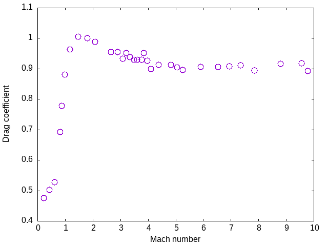
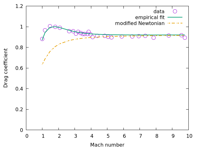
For this example we will look at comparing two models for the drag on a spherical object travelling at supersonic speed, such as a meteor. If you want to know more about drag on objects travelling at high speed you might want to look at this paper. The drag on a sphere is usually characterised in terms of a non-dimensional quantity known as the drag coefficient, which is the quantity we have tabulated in our data file. The definition of the drag coefficient is

\begin{equation}
C_D = \frac{D}{0.5 \pi \rho u^2 r^2}
\end{equation}

where \(C_D\) indicates the drag coefficient, \(\rho\) is the gas density, \(u\) is the gas velocity and \(r\) is the diameter of the sphere.

This data is saved in the comma-delimited text file ‘DragDataSpheres.csv’. The first column contains the Mach number of the flow, and the second column contains the drag coefficient.

0.22703679008802968, 0.4754504865676933
0.4289222926495784, 0.5029886144003781
0.612450731328545, 0.52777191664627
0.8164462412329196, 0.693557725580885
0.8726990369926486, 0.779240903758345
0.984149624840694, 0.8814834195623001
1.1685642666036478, 0.9643307478710026
1.4622350885781084, 1.0056430036376527
1.7918182355274597, 0.9999307917591553
2.084687254711646, 0.9887089287070719
2.651941628756867, 0.9552155161499962
2.890034857321303, 0.9550838516918039
3.0728458935037084, 0.9328629423630395
3.201345340681785, 0.9521467214705908
3.347653249833309, 0.9382409290784333
3.494045559278546, 0.9298650439303529
3.6039347416929006, 0.9298042757188796
3.7687685153144335, 0.9297131234016695
3.842365571432188, 0.951792240236996
3.97018981626056, 0.9268367613919297
4.097971860942075, 0.8991163289248247
4.372905817712245, 0.9127891765063343
4.83077741110539, 0.9125359756251952
5.05042917549353, 0.9041195783361327
5.251766076145945, 0.8957133090823157
5.892955107483774, 0.9064186423368754
6.5339753382341765, 0.9060641611032807
6.9369445405670005, 0.908606297949917
7.339913742899824, 0.9111484347965532
7.852476726619007, 0.8942751280774458
8.786872378315877, 0.9158782272562309
9.556138855363217, 0.918217803397956
9.775537418870218, 0.8932116843766618

There is an empirical formula to fit this data, and it is given by a sum of two exponentials:

\begin{equation}
C_D (M) = 2.1 e^{-1.2(M+0.35)}-8.9e^{-2.2(M+0.35)} + 0.92
\end{equation}

In hypersonic theory there is an approximate method for calculating drag, due to the great Lester Lees, called the modified Newtonian method. There’s an interesting story to Newtonian methods. As the name suggests, the model was first postulated by Isaac Newton as a way of measuring drag forces at subsonic speeds. The fluid was considered as a series of particles that hit the object like bullets fired from a gun. When the particles collide with a surface they slip along the surface, only imparting the perpendicular component of their momentum to the object. This model never really took off because it was very inaccurate at subsonic speeds. However the approximation becomes pretty good at hypersonic speeds, and so is often used as a simple way of determining the drag force, because it has the advantage of being simple to determine analytically. So I guess that proves that Newton really was ahead of his time. Lees took Newton’s idea and made a modifying calibration factor that removes an offset inherent to the model by fitting the relationship to the pressure coefficient at the stagnation point of the object, which makes it quite accurate. For a sphere, the drag can be computed using the Modified Newtonian method using the equation

\begin{equation}
C_D = \frac{1}{2} \left( \frac{2}{\gamma M^2} \left( \left[ \frac{(\gamma + 1)^2 M^2}{4 \gamma M^2 -2(\gamma-1)} \right]^{\frac{\gamma}{\gamma-1}} \left[ \frac{1-\gamma + 2 \gamma M^2}{\gamma+1} \right] -1 \right) \right)
\end{equation}

as explained in this paper.

We would like to prepare the data in J, then plot it and save it to a graphical file using Gnuplot. First, let’s just plot the first set of data from the file. The following J code sets the directory and then loads the CSV file columns into the variables M_data and CD_data.

1!:44 '/home/sean/ownCloud/Org/blog/Gnuplot/'
load 'trig plot files csv'

NB. Read the data
a =: 5 }. readcsv 'DragDataSpheres.csv'
'M_data CD_data' =: 0 ". each |:(0,1){"0 1 1 a

text =: 0 : 0
set term qt
set style data points
set datafile separator ","
set pointsize 2
plot "DragDataSpheres.csv" using 1:2 pt 6
set ylabel 'Drag coefficient'
set xlabel 'Mach number'
set nokey
pause 5
set term png
set out 'testplot.png'
rep
set out ''
set term qt
quit
)

text fwrites 'testplot.gnu'
2!:0 'gnuplot < testplot.gnu'

testplot.png

Figure 1: Drag coefficient plot

We put all of our gnuplot instructions in an adjective definition called ‘text’. The ‘pause 5’ instruction pauses for 5 seconds to give us enough time to examine the plot before it goes away. Now that we have this, we can plot our two functions

NB. C_D (M) = 2.1 e^{-1.2(M+0.35)}-8.9e^{-2.2(M+0.35)} + 0.92
CD_Fit =: (2.1 *  (^_1.2*(M_data+0.35))) - (8.9* (^_2.2*(M_data+0.35)))) + 0.92
CD_Fit

gamma =: 1.4
term1 =. 2%gamma * *: M_data
term2 =. (((*: M_data)*(*:gamma+1))%((4*gamma* *: M_data)-2*gamma-1))^gamma%gamma-1
term3 =. ((1-gamma) + 2*gamma* *: M_data)%(gamma+1)

CD_Mod_Newt =: 0.5*term1*(term2*term3)-1

(|:M_data,CD_data,CD_Fit,:CD_Mod_Newt) writecsv 'Compar.csv'

Note that I split the more complex modified Newtonian form into three separate terms before combining them. This eases debugging and also makes the probability of incorrectly parsing the right-to-left evaluation of the J code lower.

The three plots can be plotted together using the following gnuplot command…

text =: 0 : 0
set term qt
set style data points
set datafile separator ","
set pointsize 2
plot "Compar.csv" using 1:2 pt 6 t 'data', '' using 1:3 with lines lw 2 t 'empirical fit', '' using 1:4 with lines lt 4 lw 2 dashtype 2 t 'modified Newtonian'
set ylabel 'Drag coefficient'
set xlabel 'Mach number'
set yrange [0:1.2]
pause 10
set term pngcairo
set out 'Compar.png'
rep
set out ''
set term qt
quit
)

Compar2.png

Figure 2: Drag coefficient plot

Note that it’s better to use the pngcairo terminal type than png. For some reason the latter will not do dashed lines, whereas the former will.

Physically, for those interested, it shows that the modified Newtonian theory is not as good a fit as the empirical curve fit at low Mach number, but it fits the behaviour well at Mach number of 5 or greater. The curve fit won’t help you at all if the ratio of specific heats \(\gamma\) is not 1.4, but the modified Newtonian method can account for that, which makes it very useful in predicting drag.

To summarise: by loading data, doing the appropriate calculations and saving the data to a text file, we can plot the data from J using a system call to gnuplot, which will plot the raw data and any manipulations we choose to perform, combining the power of J for data analysis with the rich plotting functionality of gnuplot.

NB. Here is the full J source code

Into the Supercontinuum

Some good news: we got funded to purchase a supercontinuum IR source and a high-speed IR camera. The idea is to couple the light source into a spectrometer after being absorbed by flow, allowing for fast and easy broadband absorption spectra.

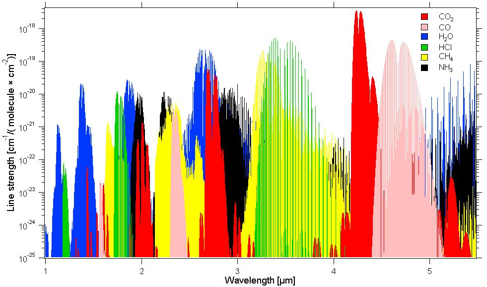
I had hoped that NKT would have an IR supercontinuum source available, but apparently they have stopped supplying it for some reason (perhaps the power was lower than they would have liked, or there may have been other problems that I’m unaware of). I have managed to find a French supplier of these sources, so hopefully I’ll still be able to do it. It would be great to be able to see entire vibrational bands of CO2 and CO with this source. CO has bands at 2.3 microns and CO2 at 2.0, and both have bands around 4-4.5 microns. If I can hit that wavelength region, I should be able to hit both species and look at Mars entry problems in this region. The really nice thing about getting so much spectral information in the IR is that you can see any vibrational nonequilibrium in the flow, and absorption is strong, so low density flows can be measured.  It may be difficult to avoid water vapour at these wavelengths, however.

from Roller et al. (2002) Applied Optics 41(28):6018.

Now I need to do the maths to make sure that we get enough absorption signal and that the source puts enough light out to be detected by the camera over the intended wavelength range, and to find the filters I need to get to limit the detected wavelengths.

This would be a good project for an Australian PhD student with an interest in laser diagnostics and hypersonics. Contact me if you are interested.

Org-babel for J

As part of my emacs org-mode work flow, I have been using org-babel for a while. This allows you to insert code blocks into org buffers and have those blocks be executed when your file is compiled. This is a really handy method for doing reproduceable research. For example, you can call the source code function in R to do the statistical calculations for data in a table. If the data in the table changes, so will the calculation of the output data change. This prevents the perennial problem of having data in one file (typically a spreadsheet) and not knowing whether the document you generated for a paper used the 12th of September or the 15th of September version of the spreadsheet. By having explicit links to data and to the algorithm that manipulates that data, you can explicitly record the calculations you used to produce your data. And so can anyone else if they want to. This is very important for producing believeable data.

Org-babel is built into emacs org-mode, and supports an amazing array of programming languages, from compiled languages like C to interpreted languages like python or MATLAB, to specialised scripting languages like awk or gnuplot.

The best feature for me is that org-mode can read from or write to org tables, allowing a seamless integration between code and document. However, this capability differs between programming languages. Some languages, like python and common lisp, seem to be very well catered for in this regard. However my favourite programming language, J, is rather less well catered for. In particular, there does not seem to be a built-in way to pass variables to and from the code block. Instead, you can run your code as if it were a script, and the source block will provide the last calculated value as an output. For example,

#+BEGIN_SRC j :exports both
 NB. The square root of the sum of the squares of the numbers
 NB. between 1 and 10
	    [a =: %: +/ *: 1 + i.10
#+END_SRC
#+RESULTS:
: 19.6214

The output, as stated by the comment, produces the Euclidean norm of the integers between 1 and 10 inclusive, which is 19.6214, and displays it as the result from evaluating the source block. However, for other programming languages one could supply a variable argument using the :var command in the header, to pass a variable argument to a function. So, for example, the 10 in the example above could be replaced by each of the values in the column of a table.

Like most things in emacs, the code for executing commands in code blocks is available as elisp. So, in theory, it should be possible to modify the existing elisp export code to pass variables, including rows and columns in tables, to a J function. At the moment though, my understanding of elisp is not sufficiently good to be able to work out how to do this, but it sounds like a very useful thing to do, and necessary if J is to be seriously used from within org-mode. If anyone has managed to do this, I’d be very interested to know how it’s done. If not, I’ll need to learn some more elisp and try to reverse engineer how it’s already been done for MATLAB code to see if I can do something equivalent for J.

Oh, and happy new year for 2021. I wanted to get one more blog entry done before the end of 2020, as an old-year’s resolution…

The Pinebook Pro

I bought a Pinebook Pro way back in November of 2019. For those who don’t know, the Pinebook Pro is an ARM64 laptop made by Pine64, a company that develops ARM64 devices and harnesses the open source software community to develop code that can drive the hardware. It’s a really interesting business model, allowing the company to focus on hardware that meets the needs of the community.

For a long time I had been keen to get an arm64 laptop. I had previously owned a couple of Odroid XU4 single-baord computers that functioned very well as a little linux box for doing basic work, but they always required an available monitor. A laptop was more convenient. For a long time, the only options were chromebook computers, which seemed to involved a lot of messing around to get Linux operating on. I bought a Teres laptop from Olimex and built it, but it was not really fast enough for my work and I had battery problems with it.  So when Pine64 announced the development of a USD199 laptop with an ARM64 processor that was designed to run Linux, and that promised a thin form factor, 4 GB RAM and 64 or 128 GB EMMC storage, I was interested.

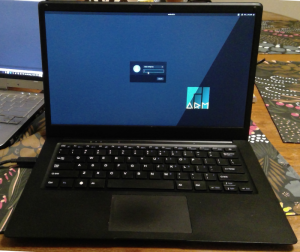
I have been using the device for about 8 months now. As an early adopter, I had the usual problems one might expext with an ARM-based linux: the trackpad was inaccurate, the device would not sleep properly, problems with wifi etc. Eventually the trackpad problems were helped by a firmware update. This was great, because the trackpad was nearly unuseable. My biggest problem was that my config files were kept on an owncloud server that was newer than the Debian version for the pineboook I was using, so I could not access these files, which were essential for my workflow. I transitioned from Debian to Manjaro, and the rolling updates solved that problem. The Manjaro folks seem to have really taken to this device, and the OS seems to work well. Figure 1 shows what the login screen looks like.

The device is plain black, with magnesium top and bottom surfaces.  The bezel and palmrest parts are plastic (more on this below).  It’s very light and the hinge is a little stiff, but holds the screen in place well. I personally like the fact that there is no logo, other than the pine logo on one of the keys that operates in place of a Windows key on a windows laptop.

Currently I am using the xfce version of Manjaro, with the i3 window manager, and I really like this combination. The regular updates get rid of many of the software problems, and about the only thing I would like would be better power consumption in sleep mode. Leaving the machine overnight in sleep mode still consumes about 70% of the battery power, which isn’t great. While working, though, I can get at least 7-8 hours use out of the device without resorting to any power reduction tricks. That’s good enough for my needs.

Figure 1: The Pinebook Pro Manjaro login screen

A couple of surprising things about this laptop: the keyboard and the screen. For $199, my expectations were certainly not high. But the screen is pretty good, with clarity and nice resolution. Also, despite the wacgrning you get when you order one of these, there were no broken pixels on it. The screen is better than the elitebooks I have used in the past, which were a lot more expensive. The keyboard is surprisingly good also, for a chiclet keyboard. It’s not a thinkpad, but it’s a lot better than a lot of other chiclet keyboards I have used, or the keyboard on my Surface Pro 4.

The wireless is not strong, but it’s OK. The bluetooth also works as well as it ever does, at least for my bluetooth headphones, and the connection struggles at times if the CPU is being used for other tasks.  The device has USB A and C ports, with the latter providing ethernet with the appropriate USB C dongle.  One other neat thing is that the wifi and camera can be turned off in hardware with some key combinations.  For those with privacy concerns, this is useful.

There are some other problematic aspects of the Pinebook Pro. Even with the firmware update, the trackpad is not very good. It’s useable, but that’s about it. The speakers are poor, and are directed under the device. But the biggest problem is the structural integrity of the device itself. The plastic is thin and brittle, and after only about a month of gentle use, cracks started to form on the wrist rests, plastic started to break around the USB ports, and eventually the plastic around the trackpad, the power barrel, and near the hinges broke from the stresses generated when the cover was opened and closed. I had the ISO keyboard. Initially I superglued the cracks and sanded the case down, which helped with some of the problems, but they got worse and worse. Figure 2 shows the damage to my keyboard, with the cracks at the power port causing problems with opening the case. If you look carefully, there are some lighter lines at the bottom left that indicate where the superglue repairs were done.  Eventually I had to buy a replacement ANSI keyboard that I installed (with firmware update) because I read on the forum that it was a better quality plastic than the plastic on the original ISO keyboard. That remains to be seen: it does not look any different to me. I suspect that I’ll have to get another keyboard in the future. The magnesium bottom and lid parts seem quite resiliant. To replace the keyboard you have to replace every board and cable on the computer, as they are screwed to the keyboard. However, I managed it, so it cannot be too hard (remember to peel the plastic from the keyboard connector). I think the physical strength of the palmrest part of the keyboard is probably the single biggest problem with this device.

One other problem for users outside the USA is that they won’t send you a replacement battery.  I suppose when the time comes I’ll need to get one from another supplier and get the wiring right.  The problem with computer batteries needing to be sent inside a computer for overseas shipping seems to me to be a cop-out.  If we are to take e-waste seriously, users should be able to easily upgrade all the components of their device, and the batteries in particular, as even rechargeable batteries are consumables.  One of the best aspects of the Pinebook Pro is that components can easily be removed for replacement and upgrade.

Figure 2: Broken ISO keyboard after disassembly

So the question I set out to answer is ‘Can the Pinebook Pro be a useful everyday computing device?’ For me, the answer is yes. For you, it may not be. It’s not a fast machine, by any means. The Surface Pro i5 runs rings around it, for example. But my needs for a computer are pretty simple. It runs Emacs, Firefox, GIMP and Inkscape well, and internet video is reasonably fast and smooth enough for YouTube. The delay is noticeable in CPU-heavy activities like compilation, but it’s not that bad. In fact, using the i3 window manager, it’s pretty zippy for the most part, with easy keyboard-based swapping between workspaces. I really like i3, and have it configured to easily provide the programs that I use on a day-to-day basis.  Like all ARM64 devices, linux applications are not as well catered for as they are for Intel CPUs, but this situation will get better with time, in particular thanks to the popularity of single-board ARM computers like the Raspberry Pi.  Despite this limitation, I’m able to do all the programming and text development needed for my scientific work on this device. I wouldn’t recommend doing CAD or playing graphical games on it, but for the text-based tasks I use linux for, it works well enough for my needs, and I really love the long battery life.  My Surface Pro lasts about 1 hour on battery after 4 years of use, and it’s nearly physically impossible to replace the battery.  In terms of hardware accessibility, the Pinebook Pro is great.

I would definitely recommend the Pinebook Pro to tinkerers like me. It’s not for those who are nervous about taking a screwdriver to their laptop, or for those who want their operating system to ‘just work’ out of the box. It is a simple and easy-to-disassemble computer.  I’ve been using it for serious work for about 6 months, and can see myself for continuing to do so, at least until the keyboard breaks again. I hope Pine64 keep improving the design and fabrication processes, developing a more robust machine that evolves with time.  I love the modular design, and the Manjaro community are doing a great job making linux work for it.  For USD199 (plus postage) this laptop’s not a bad deal at all.

DSMC in J 1

Background & Motivation

Some of my research involves flow having very low densities, or flows of moderate densities in very confined spaces, such as capillary tubes. These flows are known as rarefied flows. Rarefied flows have some interesting properties: in particular, flow can slip past boundaries, whereas at higher densities the flow would have zero velocity at a surface relative to the velocity at that surface (why cars remain dusty even when you drive them fast). In hypersonics, rarefied flows are interesting because as the flow is fast and the density is low, then fluid mechanical or chemical reaction changes can take place over similar time scales as the flow time past the object of interest. This leads to what are called nonequilibrium processes, where time scales can have an important effect on flow or on chemical reaction processes.

The DSMC Method

Because the computational solution of the fluid flow equations that treat fluids as a continuous medium assume no flow slip at surfaces, those models begin to fail when the flow gets rarefied. One very successful method for simulating rarefied flow is the direct simulation Monte Carlo (DSMC) method. This is a statistical model of flow, and was invented in the 1960s by the Australian aeronautical engineer Professor Graham Bird. I was fortunate to meet Professor Bird on several occasions later in his life (he died in 2018) and he was a very inspiring scientist. He continued to make significant contributions to rarefied flows right up to the end of his life.

DSMC is a fairly straightforward simulation method based upon a statistical treatment of collisions in rarefied gases, and because it models collisions with walls, then the slip phenomenon automatically drops out of the simulation, provided the modelling of collisions of gas atoms or molecules with the wall are physically correct. Now the most obvious way to simulate the flow of a low density gas using a computer would be to keep track of the position and momentum of every nitrogen and oxygen molecule in an air flow, step forwards in time in very small increments, calculates trajectories for each molecule during this time step to determine whether individual molecules collide with each other or with surfaces and then implement some sort of model (like Newton’s laws) for how energy and momentum are transferred for whatever collisions that occur during the time step. This idea is called Molecular Dynamics (MD). It is very useful because of its simplicity and the transparency of the physical modelling involved, but it involves too much computation for all but the smallest flow volumes and all but the lowest densities – the flow domain has to be checked at each time step for collisions between each molecule and every other molecules.

DSMC overcomes much of the problems of MD for larger flow volumes by making two very clever assumptions. The first is that the behaviour of very large collections of molecules can be simulated by considering the behaviour of a much smaller number of molecules, appropriately scaled. This alleviates the problem of dealing with astronomical numbers of physical molecules. The second assumption is that on average the behaviour of collisions between molecules can be explained by statistical means based upon knowledge of the relative speeds of the potential collision partners. Thus instead of having to solve the conservation of momentum and energy equations for each collision, the probability of collision and the post-collision trajectories can be calculated using random number generation, with the overall behaviour of the flow averaging out to the correct values. These two assumptions make DSMC capable of accurately simulating rarefied flow behaviour for a range of practical engineering problems.

I will try to explain how I split the problem up and tested the components independently as I go through the design and implementation of DSMC. The implementation will be split among various posts as I go along (and as it’s being done in my spare time, this might take a while), and I’ll discuss how I decided to attempt different solutions that didn’t work, and the struggles to get an elegant and functional loopless code. I’m not an expert in either J or DSMC, just an enthusiastic amateur. But I hope that some people will find it interesting enough to begin their own investigation of this simulation method, or be inspired to take a closer look at the frankly beautiful J programming language.

I teach a very basic version of the DSMC method to my hypersonics class, and this year I asked them to code up a simple solution as an assignment question. For this blog, I thought I would go through my method of implementing the simulation, so that those unfamiliar with molecular simulation may be tempted to try it out. To make the problem more fun for me, and because it’s a good match, I have decided to implement my solution in the J programming language. J is an array-based programming language, created by Kenneth Iverson and descended from APL, the first of the array-based languages. I chose J because, being an array-based language, it is very well suited to operation on arrays of large numbers of particles that are all doing similar things. Given that very few people know the J language, and that the intersection of those who are interested in J and are interested in DSMC has probably only one member (me) then this can be seen either as a tutorial for the J programming language that uses DSMC as an example application, or an explanation of simple DSMC that uses J as a method for describing the algorithms. My other goal in putting this together was to see if I could write some nice functional code in J that helps me cement my understanding of the DSMC method.

DSMCFlowchart.png

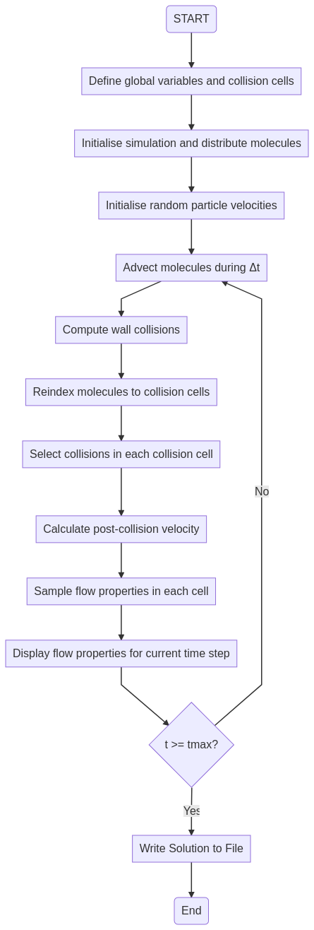
Figure 1: DSMC Flowchart

The flowchart in Fig. 1 shows the algorithm at its simplest. A representative set of molecules is uniformly distributed across the flowfield, with randomised thermal velocities superimposed upon a bulk velocity. The thermal velocities are determined using a Boltzmann distribution as a function of the initial temperature of the gas. The flowfield itself is broken up into a group of collision cells that can be of arbitrary shape or size, with a fixed number of particles within the cell. The size of the cell is therefore dependent on the local density of the flow. These particles (which I will, for convenience, call molecules regardless of whether they are molecules or atoms) are each representative of millions to billions of actual particles in the flow. A very small time step, which depends on the size of the cell, is used to determine the motion of the molecules and, along with the relative velocities of pairs of molecules, the probability of collisions. Collisions with walls and with other molecules are simulated, and the particles are re-assigned to their new cells if they move from one cell to another. After this movement, the velocities of the particles in each cell are used to determine the flow properties in the cell, and the time is incremented by Δt again. This continues until either the flow has reached a steady state or a pre-assigned time has elapsed, at which point the code stops.

As Fig. 1 and the description above indicates, the DSMC algorithm at heart is not complicated, although it should be pointed out that state-of-the-art DSMC implementations have many improvements to this simple model, to ensure that the code runs quickly and that cells or simulations are parallelised. Some real DSMC codes that you can download and use include Bird’s DS2V code or Michael Gallis’ SPARTA code, amongst others. I mention these ones specifically because they are directly downloadable so you can play with them.

There is a lot of information available in books about the DSMC method. Some references that you should look at include Prof. Bird’s original text bird1995molecular and his more recent implementation book bird2013dsmc. Other more recent texts that cover the DSMC algorithm include those by Sharipov sharipov2015rarefied and by Boyd and Schwartzentruber boyd2017nonequilibrium. We have used DSMC for validation of a number of hypersonic separated flow configurations. Some references to this work include gai2019large, le2019rotational, prakash2018direct and hruschka2011comparison.

Most of the textbooks mentioned above contain a fair amount of kinetic theory, because there is a lot of physics to be considered when dealing with collisions of molecules with each other and with surfaces. For the purposes of explaining the process of the DSMC algorithm, that extra detail is not necessary. Instead, I have used the paper by Alexander and Garcia alexander1997direct as the model for the DSMC method used here. The paper itself can be found on Prof. Alejandro Garcia’s web site (Paper), along with a lot of other interesting simulation papers. He has also written a book on numerical methods in physics which has one chapter dedicated to implementation of DSMC in Matlab or Python (or C++ or Fortran) if you prefer to avoid J or my explanations.

Over time on this blog, the plan is to implement a simple DSMC simulation in J of the flow of low density gas through a heated capillary tube of square cross-section. Each one or two steps in Fig. 1 will be implemented and described in individual blog posts, building up to the final program.

Bibliography

  • [bird1995molecular] Bird, Molecular gas dynamics and the direct simulation of gas flows, Oxford, United Kingdom: Clarendon Press(Oxford Engineering Science Series,, (42), (1995).
  • [bird2013dsmc] Bird, The DSMC method, CreateSpace Independent Publishing Platform (2013).
  • [sharipov2015rarefied] Sharipov, Rarefied gas dynamics: fundamentals for research and practice, John Wiley & Sons (2015).
  • [boyd2017nonequilibrium] Boyd & Schwartzentruber, Nonequilibrium Gas Dynamics and Molecular Simulation, Cambridge University Press (2017).
  • [gai2019large] Gai, Prakash, Khraibut, Le Page & O’Byrne, Large scale hypersonic separated flows at moderate Reynolds numbers and moderate density, 100005, in in: AIP Conference Proceedings, edited by (2019)
  • [le2019rotational] Le Page, Barrett, O’Byrne & Gai, Rotational temperature imaging of a leading-edge separation in hypervelocity flow, 110001, in in: AIP Conference Proceedings, edited by (2019)
  • [prakash2018direct] Prakash, Gai & O’Byrne, A direct simulation Monte Carlo study of hypersonic leading-edge separation with rarefaction effects, Physics of Fluids, 30(6), 063602 (2018).
  • [hruschka2011comparison] Hruschka, O’Byrne & Kleine, Comparison of velocity and temperature measurements with simulations in a hypersonic wake flow, Experiments in fluids, 51(2), 407-421 (2011).
  • [alexander1997direct] Alexander & Garcia, The direct simulation Monte Carlo method, Computers in Physics, 11(6), 588-593 (1997).

Hello, Org

This is a test blog post for writing wordpress blog items using org-mode. I’m hoping this will let me populate my blog in a more seamless manner than editing it via the WordPress web interface.

Introduction

When Ι started this blog, I got an account with an ISP and installed WordPress using some kind of automatic template. The good thing about this is that I could start a blog without knowing what I was doing. The unfortunate part about it is that when I need to configure the blog, I have no idea whatsoever about how things are set up. Also, I would need to log in to the WordPress site and use their editor to build the pages.

But what I really want to do is use org-mode directly to upload posts to my blog. As I do most of my work documentation it would be awesome to convert some of that to my web site. Fortunately some awesome person has already done the work to make this possible. It’s called Org2Blog, created by Puneeth Chaganti, and currently maintained by Grant Rettke. It’s an org-mode package that allows you to edit posts using org-mode markup and extensions. You can edit and upload the post without leaving emacs, which is great!

The remainder of this post contains some fairly useless examples of this packages capabilities.

Examples

Figure 1 is an example of html import for images. One of the nice things about org-mode is you can specify different output parameters for images in pdf and html export formats. This can be handy for making things work in HTML.

avatar image

Here is an equation, in case you ever need to know the solution to a quadratic equation:

\[ x = -b \pm \frac{\sqrt{b^2-4 a c}}{2a} \]

  • Here are some points
    • \(\LaTeX\) is great to put inline into your blog, like \(\sum_{i=0}^n i^2 = \frac{(n^2+n)(2n+1)}{6}\)
    • Centered equations use two dollar signs, as opposed to inline equations like that above, which use only one

    \[\sum_{i=0}^n i^2 = \frac{(n^2+n)(2n+1)}{6}\]

I have not yet done much to see what can be done with org-mode and wordpress. There are several things I don’t know how to do. For example, to center the image above I had to set margins, and if I were to caption it, the caption would be left aligned. I also don’t know how to number equations. References would be the next interesting thing to try hruschka2010two. Well, it seems that citations from a bibtex file will export to WordPress, but the citation style, based on the key, does not seem to change (ie I can’t get numbered or superscript citations). Nonetheless, I’m declaring the export sufficiently capable to be useful for most blog posting purposes.

Bibliography

  • [hruschka2010two] Hruschka, O’Byrne & Kleine, Two-component Doppler-shift fluorescence velocimetry applied to a generic planetary entry probe model, Experiments in Fluids, 48(6), 1109-1120 (2010).

Reminiscences on programming

I’ve just been thinking: programming computers has been a big part of my life ever since I was a child.  The first computer I ever got to touch was a microbee computer in year 7.  Before that I had seen some Atari 400s in Myer, and a TRS-80 at Tandy Electronics (Australia’s version of Radio Shack), but I was not allowed to play on them. Microbees were an Australian-made computer built specifically for the education market.  For some reason our school had two of these.  We were allowed to use some kind of word processor on it, but nobody at school seemed to know what to do with it.  I don’t remember much about it other than using it made me want a computer.  At around the same time as I was using the microbee at school, my father took early retirement from his job on the waterfront and we moved from Western Sydney to a very small town.  I was about 12.    My parents had never had much money, but they were keen on my education, and I was most likely constantly banging on about computers so one day to my amazement my Dad put down the unthinkable amount of $950 on a Commodore 64 with disk drive and 1 floppy disk, and a programmer’s reference guide and we walked out of the store with it.  I guess that once we had brought the (relatively inexpensive) house he had one shot at buying something for each of us:  Mum got an olive-green IBM Selectric typewriter, Dad got an air conditioner and a monstrous Kreisler TV with roll-out wooden doors and I got the Commodore.  Then we were poor again!

I would set the computer up in front of the big TV and spend hours with it and the programmer’s reference guide.  My father refused to buy games (having spent so much on the machine) so any games were going to have to be made by me.  My limit on the computer was around 4 hours sitting cross-legged on the floor until I would lose all feeling in my legs or Dad would make me do some outside work (the house was a fixer-upper).  I had no idea what I was doing, but I read everything I could.  During those times nothing else mattered to me.  I learned to program in BASIC, and read all the copies of Byte Magazine and Creative Computing trying (usually without success) to make the type-in basic programs work.  On the odd occasions I’d save up to purchase Australian Personal Computer or one of the many British Commodore magazines to find out more about programming.  But my town was no silicon valley, and there was no internet.  The only person I knew who knew how computers worked was the Hungarian TV repair man, who had to come in to fix a problem with Dad’s pride and joy (which I’m sure he thought my computer was responsible for creating…).  This fellow explained to me how flip-flops worked, which was to me like learning the mysteries of some secret society.

At my school we also had computers: Apple II/es in the maths department and a 32 kB BBC micro in the library.  Again, nobody seemed to know what to do with them, but I was happy to fill the void.  I think I was the only student who ever got to use the BBC micro.  It was hooked up to a Telstra-run bulletin board service called VIATEL, if I remember correctly, which was a very primitive text-based centrally served prototype for the internet.  You could check the weather, share prices and other things.  I didn’t get much of a chance to look at it, though, because they charged about 10 cents per page of text downloaded, and in the first day of playing with it, I managed to rack up a bill of around $65 in about an hour.  Before I had another chance to check my portfolio and play online poker I got called into the Vice Principal’s office and it was explained to me that I would no longer be using that computer…

We kept using the Apples, which were really nice machines.  Very sturdy construction, but only 8 colours on the display, compared to the amazing graphics and sound capability of the Commodore at home.  The sprite graphics were great.  I remember trying to program graphics on the Apple but getting nowhere.  I didn’t understand about things like memory mapping that would have really helped.  There was one older kid at the school (by the last name of Ward) who would make graphics of a sort by using lots of print statements strung together to make eg a car race track scroll down the page.  We looked down on these  ‘Wardy graphics’ programs as primitive, but at least he was able to make things that looked like animations, and he put so much time into it.

On the C64 you were limited to BASIC, although I knew that assembly language or a compiler was what all the professional programmers used.  But that stuff was certainly not readily available to me.  I think I will take to my grave the knowledge that POKE 53281,0 turned the background from the default blue to black, and that putting different numbers using the POKE command at location 53280 would do the same for the screen border.

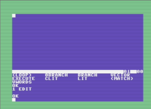
Then one fateful day in 1985 I found a cartridge in the K-mart Albury bargain bin.  It was HES Forth, an implementation of the Forth programming language for the C-64.  Not only was it a much better language than Commodore basic, with a built-in line editor, but it also had a (somewhat unusual) assembler, so that now I could finally take full advantage of a computer by converting code to machine language!  I didn’t accomplish a lot, but I learnt a lot about computers and the Forth language paradigm.  In fact, I still use that language when teaching microcontroller-based instrumentation.    I remember trying to decipher the terse user manual with all its assumed knowledge, and trying to reverse engineer a prime number generating program that they included as a demo.  That really flicked a switch somewhere in my head and programming has varied somewhere between an obsession and an interest ever since.

The line editor from HES Forth for the c64

All the programming since has been trying to recreate the thrill of making a computer do something I want it to do, delighting in working out some trick to use the computer to model something.  In hindsight I’m glad my Dad refused to buy me any games, though some of those Infocom titles did look pretty sweet at the time.  Instead I got hooked on a pastime I still get great pleasure from some 35 years later.

Over the next indefinite period when I can find the time, I’ll write up a little programming project I’ve started to model the Direct Simulation Monte Carlo method for simulating rarefied flows, using my current favourite programming language: J.  I’ll try to split the task into little parts and explain what I’m doing at each step, in case the 13-year-old version of me is listening.  I guess that’s what made me think of writing this post.

Marking pdf Assignments in Emacs

Most of the undergraduate student assignments I need to mark are numerical or analytical in nature.  The assignments are for small classes, and are often written on paper, and even if submitted electronically they are relatively easy to mark up on a tablet, because the answer is either correct or it isn’t.  But I recently had to mark a large number of assignments, for a course on the social context of engineering, where answers to questions are in paragraph form, and are fairly open-ended.  This requires explanation on my part for why marks were not allocated and suggestions on what would have made the answers better.

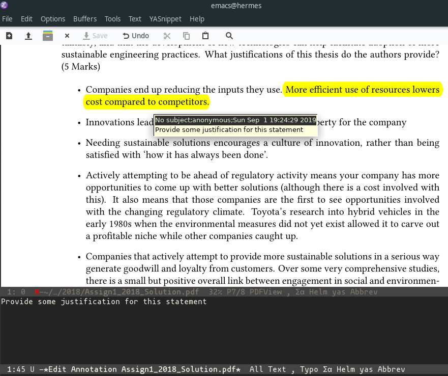
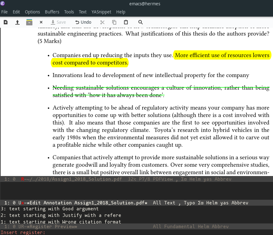
First time I did this I used a tablet and pen, and although it worked, it was very time consuming and messy to add comments.  Using Adobe Acrobat under Windows was not better, as I find the comment interface unwieldy when I have to use it a lot.  The most tedious aspect of this was that many of the comments were the same for large numbers of students, requiring you to type the same thing over and over again: this year I had around 75 students, with 6 pages and on average around 6 individual comments per page – a total of 2700 comments! Many of the mistakes were common to several students in the class.

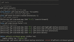
In an attempt to improve the experience of marking these assignments, I looked at doing the marking in emacs, using two very simple tools: the pdf-tools package maintained by Andreas Politz, and the built-in registers of the editor.  If you do much marking up of pdfs, this may be of interest to you.

If you use emacs, and don’t currently use pdf-tools, you should.  It’s an easy install from the melpa archive, and it is a lot faster than the default pdf viewer DocView.  Most importantly, it has commands that are useful for marking up and annotating pdf files.  I have added the following commands to my init.el file to allow single-key commands in pdf-tools such as ‘h’ for highlight text, ‘s’ for strikeout and ‘t’ for text comment, as well as ‘d’ to delete existing comments.  I also have changed the default strikeout line from red to green, because red is so judgemental…

configuration of pdf-tools

Configuration file settings for pdf-tools

When this is loaded, opening the pdf file provides a view just like that of a normal pdf-viewer, scaled to fit in the emacs window.  If I select text and hit ‘h’ I highlight that text in the pdf and get to edit a comment on the highlighted text in the minibuffer.  Pressing C-c C-c exits from the minibuffer and the comment can be seen when the cursor rolls over the highlighted text in the pdf.  Pressing ‘t’ does the same, but produces an icon in the pdf instead of the highlighted text.

Annotating in pdf-tools

Annotating in pdf-tools

Once mastered, this is a very quick way of adding comments or deleting text is very fast, as only a few keystrokes are required to add annotations, which are automatically timestamped and user stamped.  Note that I changed my user designation to anonymous here, as sometimes (eg if using for annotating review papers) it’s not desirable to identify.  By default it’s your username.

As I hinted previously, what makes this even more useful is the effectiveness in combination with emacs’ registers.  I had not really used these much previously, as I had no idea what one was supposed to do with them, but populating many pdfs with identical comments is one example of where they can be useful.

While editing a comment in the minibuffer, you can select it and type C-x-r-s-1 and it will save that text to register 1.  Then the next time you want to insert that text in a comment, you type C-x-r-i-1 and it will insert the text.  The box below gives the general idea.

Insert comment from register

Using emacs registers to recycle comments

The process can then be repeated as many times as necessary when needed in a comment.  The usual C-x C-s will save the pdf for you.  Another handy command is C-c C-a l, which lists the annotations.

This procedure is not flawless: there is a bug that comes up every so often (but not always) when editing existing annotations with pdf-tools, where the link to the animation is lost and the updated animation cannot be edited.  If this happens, kill the annotation minibuffer and make and delete another comment, then try again.  This works for me.  The only other thing I’d like to see from the excellent pdf-tools package for marking up documents is a carat symbol for insertion of text.  But I can use it perfectly well in its current form.

You can find out more about registers at https://www.emacswiki.org/emacs/Registers.

The source for pdf-tools is currently at https://github.com/politza/pdf-tools.