Getting Gnuplot Working in J
I have been trying to get Gnuplot working in J under linux. It should be easy, as there are at least two packages in J for using Gnuplot. However, it appears both of these packages presume that the user is operating the language under windows.
The motivator for this is having a way of visualising data in J. The plot package is what I would usually use, but the plot package seems to be incompatible with the i3 window manager in linux. In JQt when I try to plot something the plot window seems to be generated and then immediately vanishes. I have not been able to work out why. At least in gnuplot the window is generated and stays in place until dismissed. Using, gnuplot, although more work, also generates better-looking plots.
My particular interest is in loading, processing and plotting data files. These are usually in tab-delimited or in comma-delimited form, so let’s make an example file using the following data that gnuplot can easily read.
For this example we will look at comparing two models for the drag on a spherical object travelling at supersonic speed, such as a meteor. If you want to know more about drag on objects travelling at high speed you might want to look at this paper. The drag on a sphere is usually characterised in terms of a non-dimensional quantity known as the drag coefficient, which is the quantity we have tabulated in our data file. The definition of the drag coefficient is
\begin{equation}
C_D = \frac{D}{0.5 \pi \rho u^2 r^2}
\end{equation}
where \(C_D\) indicates the drag coefficient, \(\rho\) is the gas density, \(u\) is the gas velocity and \(r\) is the diameter of the sphere.
This data is saved in the comma-delimited text file ‘DragDataSpheres.csv’. The first column contains the Mach number of the flow, and the second column contains the drag coefficient.
0.22703679008802968, 0.4754504865676933
0.4289222926495784, 0.5029886144003781
0.612450731328545, 0.52777191664627
0.8164462412329196, 0.693557725580885
0.8726990369926486, 0.779240903758345
0.984149624840694, 0.8814834195623001
1.1685642666036478, 0.9643307478710026
1.4622350885781084, 1.0056430036376527
1.7918182355274597, 0.9999307917591553
2.084687254711646, 0.9887089287070719
2.651941628756867, 0.9552155161499962
2.890034857321303, 0.9550838516918039
3.0728458935037084, 0.9328629423630395
3.201345340681785, 0.9521467214705908
3.347653249833309, 0.9382409290784333
3.494045559278546, 0.9298650439303529
3.6039347416929006, 0.9298042757188796
3.7687685153144335, 0.9297131234016695
3.842365571432188, 0.951792240236996
3.97018981626056, 0.9268367613919297
4.097971860942075, 0.8991163289248247
4.372905817712245, 0.9127891765063343
4.83077741110539, 0.9125359756251952
5.05042917549353, 0.9041195783361327
5.251766076145945, 0.8957133090823157
5.892955107483774, 0.9064186423368754
6.5339753382341765, 0.9060641611032807
6.9369445405670005, 0.908606297949917
7.339913742899824, 0.9111484347965532
7.852476726619007, 0.8942751280774458
8.786872378315877, 0.9158782272562309
9.556138855363217, 0.918217803397956
9.775537418870218, 0.8932116843766618
There is an empirical formula to fit this data, and it is given by a sum of two exponentials:
\begin{equation}
C_D (M) = 2.1 e^{-1.2(M+0.35)}-8.9e^{-2.2(M+0.35)} + 0.92
\end{equation}
In hypersonic theory there is an approximate method for calculating drag, due to the great Lester Lees, called the modified Newtonian method. There’s an interesting story to Newtonian methods. As the name suggests, the model was first postulated by Isaac Newton as a way of measuring drag forces at subsonic speeds. The fluid was considered as a series of particles that hit the object like bullets fired from a gun. When the particles collide with a surface they slip along the surface, only imparting the perpendicular component of their momentum to the object. This model never really took off because it was very inaccurate at subsonic speeds. However the approximation becomes pretty good at hypersonic speeds, and so is often used as a simple way of determining the drag force, because it has the advantage of being simple to determine analytically. So I guess that proves that Newton really was ahead of his time. Lees took Newton’s idea and made a modifying calibration factor that removes an offset inherent to the model by fitting the relationship to the pressure coefficient at the stagnation point of the object, which makes it quite accurate. For a sphere, the drag can be computed using the Modified Newtonian method using the equation
\begin{equation}
C_D = \frac{1}{2} \left( \frac{2}{\gamma M^2} \left( \left[ \frac{(\gamma + 1)^2 M^2}{4 \gamma M^2 -2(\gamma-1)} \right]^{\frac{\gamma}{\gamma-1}} \left[ \frac{1-\gamma + 2 \gamma M^2}{\gamma+1} \right] -1 \right) \right)
\end{equation}
as explained in this paper.
We would like to prepare the data in J, then plot it and save it to a graphical file using Gnuplot. First, let’s just plot the first set of data from the file. The following J code sets the directory and then loads the CSV file columns into the variables M_data and CD_data.
1!:44 '/home/sean/ownCloud/Org/blog/Gnuplot/'
load 'trig plot files csv'

NB. Read the data
a =: 5 }. readcsv 'DragDataSpheres.csv'
'M_data CD_data' =: 0 ". each |:(0,1){"0 1 1 a

text =: 0 : 0
set term qt
set style data points
set datafile separator ","
set pointsize 2
plot "DragDataSpheres.csv" using 1:2 pt 6
set ylabel 'Drag coefficient'
set xlabel 'Mach number'
set nokey
pause 5
set term png
set out 'testplot.png'
rep
set out ''
set term qt
quit
)

text fwrites 'testplot.gnu'
2!:0 'gnuplot < testplot.gnu'
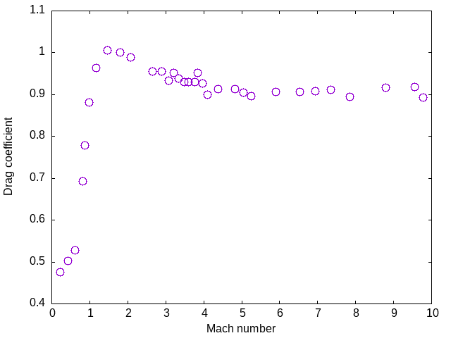
Figure 1: Drag coefficient plot
We put all of our gnuplot instructions in an adjective definition called ‘text’. The ‘pause 5’ instruction pauses for 5 seconds to give us enough time to examine the plot before it goes away. Now that we have this, we can plot our two functions
NB. C_D (M) = 2.1 e^{-1.2(M+0.35)}-8.9e^{-2.2(M+0.35)} + 0.92
CD_Fit =: (2.1 *  (^_1.2*(M_data+0.35))) - (8.9* (^_2.2*(M_data+0.35)))) + 0.92
CD_Fit

gamma =: 1.4
term1 =. 2%gamma * *: M_data
term2 =. (((*: M_data)*(*:gamma+1))%((4*gamma* *: M_data)-2*gamma-1))^gamma%gamma-1
term3 =. ((1-gamma) + 2*gamma* *: M_data)%(gamma+1)

CD_Mod_Newt =: 0.5*term1*(term2*term3)-1

(|:M_data,CD_data,CD_Fit,:CD_Mod_Newt) writecsv 'Compar.csv'
Note that I split the more complex modified Newtonian form into three separate terms before combining them. This eases debugging and also makes the probability of incorrectly parsing the right-to-left evaluation of the J code lower.
The three plots can be plotted together using the following gnuplot command…
text =: 0 : 0
set term qt
set style data points
set datafile separator ","
set pointsize 2
plot "Compar.csv" using 1:2 pt 6 t 'data', '' using 1:3 with lines lw 2 t 'empirical fit', '' using 1:4 with lines lt 4 lw 2 dashtype 2 t 'modified Newtonian'
set ylabel 'Drag coefficient'
set xlabel 'Mach number'
set yrange [0:1.2]
pause 10
set term pngcairo
set out 'Compar.png'
rep
set out ''
set term qt
quit
)
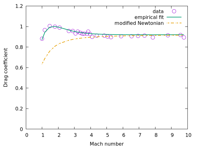
Figure 2: Drag coefficient plot
Note that it’s better to use the pngcairo terminal type than png. For some reason the latter will not do dashed lines, whereas the former will.
Physically, for those interested, it shows that the modified Newtonian theory is not as good a fit as the empirical curve fit at low Mach number, but it fits the behaviour well at Mach number of 5 or greater. The curve fit won’t help you at all if the ratio of specific heats \(\gamma\) is not 1.4, but the modified Newtonian method can account for that, which makes it very useful in predicting drag.
To summarise: by loading data, doing the appropriate calculations and saving the data to a text file, we can plot the data from J using a system call to gnuplot, which will plot the raw data and any manipulations we choose to perform, combining the power of J for data analysis with the rich plotting functionality of gnuplot.
NB. Here is the full J source code
Leave a Reply