HyperScience

New Daily Driver: the Odroid N2+

I have always had a soft spot for fanless ARM single-board computers (SBCs) because they are quiet, portable and consume very little power compared to a typical laptop or desktop machine. A typical desktop computer will consume from 100 to 500 Watts of power, while a typical laptop consumes 60 to 90 Watts. An ARM SBC can consume anything from 6 to 30 Watts, which is considerably less than either of the more common formats. They also have less in the way of hardware monitoring than intel-based CPUs, and can run linux, which is my preferred operating system.

Until fairly recently, however, these machines have been too slow to operate well as standard work computers because package availability was sloppy and memory and CPU availability were at the low end of what you would typically need to get the job done. Also graphic processor support, the bane of linux, is particularly bad for these devices, as they tend to have commercial GPU drivers (as phones are their main application market).

As I mostly use open-source software for my research, and my graphical needs are fairly simple, I have proved to my own satisfaction that I can use these boards to do real work, albeit with a performance penalty compared to a modern i5 or i7 intel chip laptop. My first arm machine was an Odroid XU4 which I brought with me on sabbatical and used for writing papers and reports over a 5-month period. The only problem I had with that machine was that it would get into funny states after updating the OS, and it required a fan. Subsequent to this, I purchased a Pinebook Pro, which I could use as a laptop but which was a slower than the XU4, making the experience a little too frustrating to persevere with in the longer term, though I still use it from time to time.

Now Hardkernal, the maker of the odroid machines, has a new ARM64 SBC which is more powerful than the XU4, the Odroid N2+. This device is marketed as an alternative to the Raspberry pi 4 (which I have not used), being more powerful and more expensive. I purchased mine for USD86 with a plastic case, wireless dongle, and 128 GB emmc card (note that if you are going to use a computer seriously, having as much solid state storage as possible is very helpful). The device comes with 4GB of memory which, as the old Rolls-Royce acceleration specs used to say, is `adequate’.

This device uses more power than the XU4, requiring 12V and 2 A, rather than 5V at 3A. But this is not so surprising given the extra speed of the newer device. It also is by default fanless, although a fan is available for high load applications. So far in using it for my work, the heatsink has not got much more than warm. Although the device can apparently be overclocked to 2.4 GHz, I have not attempted overclocking it.

Initially if you purchase the device from the hardkernel web site, the emmc chip comes with ubuntu mate installed as the recommended operating system. As I like manjaro better than ubuntu, after playing around a bit with the default I used etcher to implement a manjaro sway windowing environment that has been compiled specifically for this computer. After a successful install I noticed that the screen I was using with the N2+ (a QHD 32″ lenovo monitor) would flicker randomly, which was very irritating. In case it was a problem with the Wayland system, I installed manjaro XFCE, which uses X11 rather than Wayland, but when I tried the XFCE version of manjaro, the flickering still occurred. So after a couple of unsuccessful installs, I went back to the original Ubuntu mate installation, which does not cause the flicker problem on my monitor, presumably because hardkernel installed the correct graphics drivers.

I really like tiling window managers that you can control via the keyboard (hence my initial desire to use sway), so once I had mate installed and the default user account removed I installed i3. The i3 window manager seems to work really well under ubuntu, and I was able to set things up just the way I like them. One of the things I don’t like about ubuntu and other Debian-based distributions is the slow turnaround time, as several applications require very up-to-date versions to operate properly (like my University’s owncloud server). However I was pleasantly surprised this time that most programs installable by apt were able to work without causing me problems because of their age.

Here is a picture of what the configuration looks like. The image shows emacs, a translucent shell window (terminator, using powershell) and a web browser all open on the same workspace. The little icons on the bottom right show the other three workspaces that can be used.

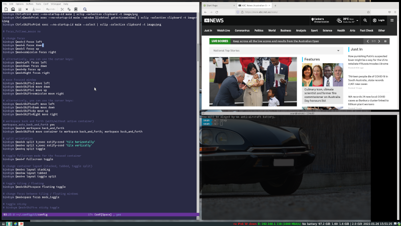
Figure 1: i3 configuration

Because i3 is pretty lightweight compared to many window managers, the transition between workspaces and switching between applications is very fast. Using the emacs daemon makes editing very fast too. Once you get used to it, the keyboard-driven workflow associated with i3 and emacs is pretty hard to beat.

In total, with the blind alleys caused by trying the other distros, it took about 10 hours to completely set up the N2 the way I want it. Now I can use all the tools that I use on the intel laptop for my research work, and apart from taking a little longer to load programs, I don’t experience much lag at all compared to my i7 laptop. I was able to connect to my cloud service and to run all the codes I need to, either using snaps, apt, or in a couple of cases compiling from source. The experience is no worse than my usual linux installation experience (best described as me trying lots of permutations of random things based upon internet searches until something works). My existing i3 and emacs configurations were basically able to be transferred directly to the new computer with very few changes necessary. Because all my work in progress is on the cloud, this means that I can work on my project either on my laptop or on this SBC with seamless results, as I have the same applications installed on both machines.

In summary, I’m impressed. This blog post was written on it using emacs org2blog.  It’s possible that I might get bored or frustrated and stop using this machine for work, in which case it will be used as a lab device for transferring data from instruments, or as a connected diary device.  But at the moment I can’t much tell the difference between working on this machine and working on my laptop, and that’s a very good sign.  It’s really impressive how far ARM64 support has come in linux.  For a total outlay of less than AUD200, this is a really fun-to-use laptop replacement, provided you have access to a HDMI monitor and as long as you don’t mind shutting it down between moves (because it does not have a battery).  4GB is not a lot of memory, but in linux I have yet to reach a limit that affects my work in terms of available memory.

The small size of this machine means that, with a big rechargeable battery, it could be made into a very nice portable computer provided you have access to a TV or monitor with HDMI support, which is pretty much everything these days.  I have some ideas about form factors that I hope to have time to try out one day…

First Reproducible Research Paper

I have been playing around with reproducible research in org-mode. As an example for students, I have produced a paper written entirely in org-mode and containing all the required calculations within the document itself. The diagram was made using DITAA and the values were calculated and plotted using calls to elisp and python routines. The paper is formatted as if if were a paper in the Springer Journal Shock Waves, as I wanted to demonstrate the ease of using org-mode with a \(\LaTeX\) style for journal papers. It should be possible, though not necessarily straightforward, to change the style to suit whatever form of journal paper was required. I just chose this one because I like the Springer journal format and fonts.

The paper is on the eternal problem of whether your tea will be cooler after 10 minutes if you mix the milk and the tea immediately and then waiting 10 minutes or by waiting and then adding the tea. You’ll have to read the paper to find out the answer! This is a simple enough problem that allows for a demonstration of how equations and figures are generated and presented using the org-mode markup features.

It was an interesting experience to write this paper. It took me around 2 days of full-time work to get it up and running, but now that I’ve done it, the process should be much quicker for an actual paper. It was not always straightforward to get working either: I found the referencing of figures and tables was hit-and-miss. I’m not sure whether this is normal, or something to do with my configuration, but I often found myself looking at and compiling the .tex files produced by org to determine where my labels ended up and why they were sometimes not found. But eventually I did get it working.

My knowledge of python was not really good enough to allow me to do much in the way of calculating and plotting data, and I was not able to work out how to call a python routine to put numbers in a table. I therefore decided to do most of the table calculations in elisp, where the interface to the org-table is quite seamless. Although I find mathematics in lisp a little awkward, I was able to get it all working with a minimum of fuss, and elisp is pretty easy to debug in emacs.

It’s certainly very neat to be able to populate the text with computed numbers that can change whenever the input parameters for the paper change. And having the plots automatically update when the data is changed is also wonderful. For me, this is the way to properly write a paper, even though there is certainly more groundwork that needs to be done to get the paper written. It may not also work so well for papers where there is a lot of computational work, or where commercial gui-based software is used. But most of my papers contain only small calculations using scripting languages called from the command-line, and org-mode is perfect for that workflow.

An annoyance that I was not expecting is that for the Springer journal file, the abstract occurs in the preamble, so I could not just include a bunch of #+LATEX_HEADER: commands. Instead I needed to use a \input command to include the \(\LaTeX\) within the document.

My plan is for this paper to form a template for a document on how to set up emacs and org-mode from scratch in a new linux distribution, so any student gets a head-start in how to make a reproducible research paper. I could have added more bells and whistles, but I deliberately chose a minimal useful set to not cause unnecessary confusion.

Here is the pdf of the paper

Here is the org-mode file

Here is the bibliography file

Here is the \(\LaTeX\) header file

Because of the wordpress limits on file extensions I had to change all but the pdf file to a .txt extension.

Sometime soon I plan to write the installation from scratch document that allows one to go from a new installation of ubuntu to being able to produce this document.

Getting Gnuplot Working in J

I have been trying to get Gnuplot working in J under linux. It should be easy, as there are at least two packages in J for using Gnuplot. However, it appears both of these packages presume that the user is operating the language under windows.

The motivator for this is having a way of visualising data in J. The plot package is what I would usually use, but the plot package seems to be incompatible with the i3 window manager in linux. In JQt when I try to plot something the plot window seems to be generated and then immediately vanishes. I have not been able to work out why. At least in gnuplot the window is generated and stays in place until dismissed. Using, gnuplot, although more work, also generates better-looking plots.

My particular interest is in loading, processing and plotting data files. These are usually in tab-delimited or in comma-delimited form, so let’s make an example file using the following data that gnuplot can easily read.

For this example we will look at comparing two models for the drag on a spherical object travelling at supersonic speed, such as a meteor. If you want to know more about drag on objects travelling at high speed you might want to look at this paper. The drag on a sphere is usually characterised in terms of a non-dimensional quantity known as the drag coefficient, which is the quantity we have tabulated in our data file. The definition of the drag coefficient is

\begin{equation}
C_D = \frac{D}{0.5 \pi \rho u^2 r^2}
\end{equation}

where \(C_D\) indicates the drag coefficient, \(\rho\) is the gas density, \(u\) is the gas velocity and \(r\) is the diameter of the sphere.

This data is saved in the comma-delimited text file ‘DragDataSpheres.csv’. The first column contains the Mach number of the flow, and the second column contains the drag coefficient.

0.22703679008802968, 0.4754504865676933
0.4289222926495784, 0.5029886144003781
0.612450731328545, 0.52777191664627
0.8164462412329196, 0.693557725580885
0.8726990369926486, 0.779240903758345
0.984149624840694, 0.8814834195623001
1.1685642666036478, 0.9643307478710026
1.4622350885781084, 1.0056430036376527
1.7918182355274597, 0.9999307917591553
2.084687254711646, 0.9887089287070719
2.651941628756867, 0.9552155161499962
2.890034857321303, 0.9550838516918039
3.0728458935037084, 0.9328629423630395
3.201345340681785, 0.9521467214705908
3.347653249833309, 0.9382409290784333
3.494045559278546, 0.9298650439303529
3.6039347416929006, 0.9298042757188796
3.7687685153144335, 0.9297131234016695
3.842365571432188, 0.951792240236996
3.97018981626056, 0.9268367613919297
4.097971860942075, 0.8991163289248247
4.372905817712245, 0.9127891765063343
4.83077741110539, 0.9125359756251952
5.05042917549353, 0.9041195783361327
5.251766076145945, 0.8957133090823157
5.892955107483774, 0.9064186423368754
6.5339753382341765, 0.9060641611032807
6.9369445405670005, 0.908606297949917
7.339913742899824, 0.9111484347965532
7.852476726619007, 0.8942751280774458
8.786872378315877, 0.9158782272562309
9.556138855363217, 0.918217803397956
9.775537418870218, 0.8932116843766618

There is an empirical formula to fit this data, and it is given by a sum of two exponentials:

\begin{equation}
C_D (M) = 2.1 e^{-1.2(M+0.35)}-8.9e^{-2.2(M+0.35)} + 0.92
\end{equation}

In hypersonic theory there is an approximate method for calculating drag, due to the great Lester Lees, called the modified Newtonian method. There’s an interesting story to Newtonian methods. As the name suggests, the model was first postulated by Isaac Newton as a way of measuring drag forces at subsonic speeds. The fluid was considered as a series of particles that hit the object like bullets fired from a gun. When the particles collide with a surface they slip along the surface, only imparting the perpendicular component of their momentum to the object. This model never really took off because it was very inaccurate at subsonic speeds. However the approximation becomes pretty good at hypersonic speeds, and so is often used as a simple way of determining the drag force, because it has the advantage of being simple to determine analytically. So I guess that proves that Newton really was ahead of his time. Lees took Newton’s idea and made a modifying calibration factor that removes an offset inherent to the model by fitting the relationship to the pressure coefficient at the stagnation point of the object, which makes it quite accurate. For a sphere, the drag can be computed using the Modified Newtonian method using the equation

\begin{equation}
C_D = \frac{1}{2} \left( \frac{2}{\gamma M^2} \left( \left[ \frac{(\gamma + 1)^2 M^2}{4 \gamma M^2 -2(\gamma-1)} \right]^{\frac{\gamma}{\gamma-1}} \left[ \frac{1-\gamma + 2 \gamma M^2}{\gamma+1} \right] -1 \right) \right)
\end{equation}

as explained in this paper.

We would like to prepare the data in J, then plot it and save it to a graphical file using Gnuplot. First, let’s just plot the first set of data from the file. The following J code sets the directory and then loads the CSV file columns into the variables M_data and CD_data.

1!:44 '/home/sean/ownCloud/Org/blog/Gnuplot/'
load 'trig plot files csv'

NB. Read the data
a =: 5 }. readcsv 'DragDataSpheres.csv'
'M_data CD_data' =: 0 ". each |:(0,1){"0 1 1 a

text =: 0 : 0
set term qt
set style data points
set datafile separator ","
set pointsize 2
plot "DragDataSpheres.csv" using 1:2 pt 6
set ylabel 'Drag coefficient'
set xlabel 'Mach number'
set nokey
pause 5
set term png
set out 'testplot.png'
rep
set out ''
set term qt
quit
)

text fwrites 'testplot.gnu'
2!:0 'gnuplot < testplot.gnu'

testplot.png

Figure 1: Drag coefficient plot

We put all of our gnuplot instructions in an adjective definition called ‘text’. The ‘pause 5’ instruction pauses for 5 seconds to give us enough time to examine the plot before it goes away. Now that we have this, we can plot our two functions

NB. C_D (M) = 2.1 e^{-1.2(M+0.35)}-8.9e^{-2.2(M+0.35)} + 0.92
CD_Fit =: (2.1 *  (^_1.2*(M_data+0.35))) - (8.9* (^_2.2*(M_data+0.35)))) + 0.92
CD_Fit

gamma =: 1.4
term1 =. 2%gamma * *: M_data
term2 =. (((*: M_data)*(*:gamma+1))%((4*gamma* *: M_data)-2*gamma-1))^gamma%gamma-1
term3 =. ((1-gamma) + 2*gamma* *: M_data)%(gamma+1)

CD_Mod_Newt =: 0.5*term1*(term2*term3)-1

(|:M_data,CD_data,CD_Fit,:CD_Mod_Newt) writecsv 'Compar.csv'

Note that I split the more complex modified Newtonian form into three separate terms before combining them. This eases debugging and also makes the probability of incorrectly parsing the right-to-left evaluation of the J code lower.

The three plots can be plotted together using the following gnuplot command…

text =: 0 : 0
set term qt
set style data points
set datafile separator ","
set pointsize 2
plot "Compar.csv" using 1:2 pt 6 t 'data', '' using 1:3 with lines lw 2 t 'empirical fit', '' using 1:4 with lines lt 4 lw 2 dashtype 2 t 'modified Newtonian'
set ylabel 'Drag coefficient'
set xlabel 'Mach number'
set yrange [0:1.2]
pause 10
set term pngcairo
set out 'Compar.png'
rep
set out ''
set term qt
quit
)

Compar2.png

Figure 2: Drag coefficient plot

Note that it’s better to use the pngcairo terminal type than png. For some reason the latter will not do dashed lines, whereas the former will.

Physically, for those interested, it shows that the modified Newtonian theory is not as good a fit as the empirical curve fit at low Mach number, but it fits the behaviour well at Mach number of 5 or greater. The curve fit won’t help you at all if the ratio of specific heats \(\gamma\) is not 1.4, but the modified Newtonian method can account for that, which makes it very useful in predicting drag.

To summarise: by loading data, doing the appropriate calculations and saving the data to a text file, we can plot the data from J using a system call to gnuplot, which will plot the raw data and any manipulations we choose to perform, combining the power of J for data analysis with the rich plotting functionality of gnuplot.

NB. Here is the full J source code

Into the Supercontinuum

Some good news: we got funded to purchase a supercontinuum IR source and a high-speed IR camera. The idea is to couple the light source into a spectrometer after being absorbed by flow, allowing for fast and easy broadband absorption spectra.

I had hoped that NKT would have an IR supercontinuum source available, but apparently they have stopped supplying it for some reason (perhaps the power was lower than they would have liked, or there may have been other problems that I’m unaware of). I have managed to find a French supplier of these sources, so hopefully I’ll still be able to do it. It would be great to be able to see entire vibrational bands of CO2 and CO with this source. CO has bands at 2.3 microns and CO2 at 2.0, and both have bands around 4-4.5 microns. If I can hit that wavelength region, I should be able to hit both species and look at Mars entry problems in this region. The really nice thing about getting so much spectral information in the IR is that you can see any vibrational nonequilibrium in the flow, and absorption is strong, so low density flows can be measured.  It may be difficult to avoid water vapour at these wavelengths, however.

from Roller et al. (2002) Applied Optics 41(28):6018.

Now I need to do the maths to make sure that we get enough absorption signal and that the source puts enough light out to be detected by the camera over the intended wavelength range, and to find the filters I need to get to limit the detected wavelengths.

This would be a good project for an Australian PhD student with an interest in laser diagnostics and hypersonics. Contact me if you are interested.

DSMC in J 1

Background & Motivation

Some of my research involves flow having very low densities, or flows of moderate densities in very confined spaces, such as capillary tubes. These flows are known as rarefied flows. Rarefied flows have some interesting properties: in particular, flow can slip past boundaries, whereas at higher densities the flow would have zero velocity at a surface relative to the velocity at that surface (why cars remain dusty even when you drive them fast). In hypersonics, rarefied flows are interesting because as the flow is fast and the density is low, then fluid mechanical or chemical reaction changes can take place over similar time scales as the flow time past the object of interest. This leads to what are called nonequilibrium processes, where time scales can have an important effect on flow or on chemical reaction processes.

The DSMC Method

Because the computational solution of the fluid flow equations that treat fluids as a continuous medium assume no flow slip at surfaces, those models begin to fail when the flow gets rarefied. One very successful method for simulating rarefied flow is the direct simulation Monte Carlo (DSMC) method. This is a statistical model of flow, and was invented in the 1960s by the Australian aeronautical engineer Professor Graham Bird. I was fortunate to meet Professor Bird on several occasions later in his life (he died in 2018) and he was a very inspiring scientist. He continued to make significant contributions to rarefied flows right up to the end of his life.

DSMC is a fairly straightforward simulation method based upon a statistical treatment of collisions in rarefied gases, and because it models collisions with walls, then the slip phenomenon automatically drops out of the simulation, provided the modelling of collisions of gas atoms or molecules with the wall are physically correct. Now the most obvious way to simulate the flow of a low density gas using a computer would be to keep track of the position and momentum of every nitrogen and oxygen molecule in an air flow, step forwards in time in very small increments, calculates trajectories for each molecule during this time step to determine whether individual molecules collide with each other or with surfaces and then implement some sort of model (like Newton’s laws) for how energy and momentum are transferred for whatever collisions that occur during the time step. This idea is called Molecular Dynamics (MD). It is very useful because of its simplicity and the transparency of the physical modelling involved, but it involves too much computation for all but the smallest flow volumes and all but the lowest densities – the flow domain has to be checked at each time step for collisions between each molecule and every other molecules.

DSMC overcomes much of the problems of MD for larger flow volumes by making two very clever assumptions. The first is that the behaviour of very large collections of molecules can be simulated by considering the behaviour of a much smaller number of molecules, appropriately scaled. This alleviates the problem of dealing with astronomical numbers of physical molecules. The second assumption is that on average the behaviour of collisions between molecules can be explained by statistical means based upon knowledge of the relative speeds of the potential collision partners. Thus instead of having to solve the conservation of momentum and energy equations for each collision, the probability of collision and the post-collision trajectories can be calculated using random number generation, with the overall behaviour of the flow averaging out to the correct values. These two assumptions make DSMC capable of accurately simulating rarefied flow behaviour for a range of practical engineering problems.

I will try to explain how I split the problem up and tested the components independently as I go through the design and implementation of DSMC. The implementation will be split among various posts as I go along (and as it’s being done in my spare time, this might take a while), and I’ll discuss how I decided to attempt different solutions that didn’t work, and the struggles to get an elegant and functional loopless code. I’m not an expert in either J or DSMC, just an enthusiastic amateur. But I hope that some people will find it interesting enough to begin their own investigation of this simulation method, or be inspired to take a closer look at the frankly beautiful J programming language.

I teach a very basic version of the DSMC method to my hypersonics class, and this year I asked them to code up a simple solution as an assignment question. For this blog, I thought I would go through my method of implementing the simulation, so that those unfamiliar with molecular simulation may be tempted to try it out. To make the problem more fun for me, and because it’s a good match, I have decided to implement my solution in the J programming language. J is an array-based programming language, created by Kenneth Iverson and descended from APL, the first of the array-based languages. I chose J because, being an array-based language, it is very well suited to operation on arrays of large numbers of particles that are all doing similar things. Given that very few people know the J language, and that the intersection of those who are interested in J and are interested in DSMC has probably only one member (me) then this can be seen either as a tutorial for the J programming language that uses DSMC as an example application, or an explanation of simple DSMC that uses J as a method for describing the algorithms. My other goal in putting this together was to see if I could write some nice functional code in J that helps me cement my understanding of the DSMC method.

DSMCFlowchart.png

Figure 1: DSMC Flowchart

The flowchart in Fig. 1 shows the algorithm at its simplest. A representative set of molecules is uniformly distributed across the flowfield, with randomised thermal velocities superimposed upon a bulk velocity. The thermal velocities are determined using a Boltzmann distribution as a function of the initial temperature of the gas. The flowfield itself is broken up into a group of collision cells that can be of arbitrary shape or size, with a fixed number of particles within the cell. The size of the cell is therefore dependent on the local density of the flow. These particles (which I will, for convenience, call molecules regardless of whether they are molecules or atoms) are each representative of millions to billions of actual particles in the flow. A very small time step, which depends on the size of the cell, is used to determine the motion of the molecules and, along with the relative velocities of pairs of molecules, the probability of collisions. Collisions with walls and with other molecules are simulated, and the particles are re-assigned to their new cells if they move from one cell to another. After this movement, the velocities of the particles in each cell are used to determine the flow properties in the cell, and the time is incremented by Δt again. This continues until either the flow has reached a steady state or a pre-assigned time has elapsed, at which point the code stops.

As Fig. 1 and the description above indicates, the DSMC algorithm at heart is not complicated, although it should be pointed out that state-of-the-art DSMC implementations have many improvements to this simple model, to ensure that the code runs quickly and that cells or simulations are parallelised. Some real DSMC codes that you can download and use include Bird’s DS2V code or Michael Gallis’ SPARTA code, amongst others. I mention these ones specifically because they are directly downloadable so you can play with them.

There is a lot of information available in books about the DSMC method. Some references that you should look at include Prof. Bird’s original text bird1995molecular and his more recent implementation book bird2013dsmc. Other more recent texts that cover the DSMC algorithm include those by Sharipov sharipov2015rarefied and by Boyd and Schwartzentruber boyd2017nonequilibrium. We have used DSMC for validation of a number of hypersonic separated flow configurations. Some references to this work include gai2019large, le2019rotational, prakash2018direct and hruschka2011comparison.

Most of the textbooks mentioned above contain a fair amount of kinetic theory, because there is a lot of physics to be considered when dealing with collisions of molecules with each other and with surfaces. For the purposes of explaining the process of the DSMC algorithm, that extra detail is not necessary. Instead, I have used the paper by Alexander and Garcia alexander1997direct as the model for the DSMC method used here. The paper itself can be found on Prof. Alejandro Garcia’s web site (Paper), along with a lot of other interesting simulation papers. He has also written a book on numerical methods in physics which has one chapter dedicated to implementation of DSMC in Matlab or Python (or C++ or Fortran) if you prefer to avoid J or my explanations.

Over time on this blog, the plan is to implement a simple DSMC simulation in J of the flow of low density gas through a heated capillary tube of square cross-section. Each one or two steps in Fig. 1 will be implemented and described in individual blog posts, building up to the final program.

Bibliography

  • [bird1995molecular] Bird, Molecular gas dynamics and the direct simulation of gas flows, Oxford, United Kingdom: Clarendon Press(Oxford Engineering Science Series,, (42), (1995).
  • [bird2013dsmc] Bird, The DSMC method, CreateSpace Independent Publishing Platform (2013).
  • [sharipov2015rarefied] Sharipov, Rarefied gas dynamics: fundamentals for research and practice, John Wiley & Sons (2015).
  • [boyd2017nonequilibrium] Boyd & Schwartzentruber, Nonequilibrium Gas Dynamics and Molecular Simulation, Cambridge University Press (2017).
  • [gai2019large] Gai, Prakash, Khraibut, Le Page & O’Byrne, Large scale hypersonic separated flows at moderate Reynolds numbers and moderate density, 100005, in in: AIP Conference Proceedings, edited by (2019)
  • [le2019rotational] Le Page, Barrett, O’Byrne & Gai, Rotational temperature imaging of a leading-edge separation in hypervelocity flow, 110001, in in: AIP Conference Proceedings, edited by (2019)
  • [prakash2018direct] Prakash, Gai & O’Byrne, A direct simulation Monte Carlo study of hypersonic leading-edge separation with rarefaction effects, Physics of Fluids, 30(6), 063602 (2018).
  • [hruschka2011comparison] Hruschka, O’Byrne & Kleine, Comparison of velocity and temperature measurements with simulations in a hypersonic wake flow, Experiments in fluids, 51(2), 407-421 (2011).
  • [alexander1997direct] Alexander & Garcia, The direct simulation Monte Carlo method, Computers in Physics, 11(6), 588-593 (1997).